Workshop: MBA
In the lecture we discussed that association rule mining encompasses a broad set of analytics techniques aimed at uncovering the associations and connections between specific objects. It was initially used for Market Basket Analysis (MBA) to find how items purchased by customers are associated. This exercise is based on MBA. You will gain better understanding of the three strength of rule measures - support, confidence and lift. If we have enough time, we will explore how to create a transaction data file in the last exercise.
There are two major packages that are often used for performing market basket analysis (MBA) in R: arules and arulesViz. The former contain a function apriori() which is used to identify the association rules while the latter is used to visualise these rules. We will require additional package such as dplyr and stringr for the exercises.
It is worth mentioning again that apriori algorithm uses a level-wise search, where \(k\)-itemsets are used to explore (\(k+1\))-itemsets. Frequent subsets are extended one item at a time and then groups of candidates are tested against the data. It is computationally fast since it takes advantage of the fact that any subset of a frequent itemset is also frequent. This reduces the number of candidates being considered by only exploring the itemsets whose support count is greater than the minimum support count.
BreadBasket_DMS data
We will carryout market basket analysis with the apriori algorithm using the Bakery data set. The dataset consists of 21293 observations from a bakery. The data file contains four variables, Date, Time, Transaction ID and Item. Transaction ID ranges from 1 through 9684. However, there are some skipped numbers in Transaction IDs. A copy of the data is available in the file BreadBasket_DMS.csv on Ultra. For further information about the data, please see the Kaggle website HERE.
Before reading the data into R as a transaction data set, we may need to explore the data first by using some data wrangling techniques.
trans_csv <- read.csv('BreadBasket_DMS.csv',sep=",")
str(trans_csv)
## 'data.frame': 21293 obs. of 4 variables:
## $ Date : chr "2016-10-30" "2016-10-30" "2016-10-30" "2016-10-30" ...
## $ Time : chr "09:58:11" "10:05:34" "10:05:34" "10:07:57" ...
## $ Transaction: int 1 2 2 3 3 3 4 5 5 5 ...
## $ Item : chr "Bread" "Scandinavian" "Scandinavian" "Hot chocolate" ...
Let’s take a glimpse into the data.
head(trans_csv)## Date Time Transaction Item
## 1 2016-10-30 09:58:11 1 Bread
## 2 2016-10-30 10:05:34 2 Scandinavian
## 3 2016-10-30 10:05:34 2 Scandinavian
## 4 2016-10-30 10:07:57 3 Hot chocolate
## 5 2016-10-30 10:07:57 3 Jam
## 6 2016-10-30 10:07:57 3 Cookiesnames(trans_csv)## [1] "Date" "Time" "Transaction" "Item"unique(trans_csv$Item)## [1] "Bread" "Scandinavian"
## [3] "Hot chocolate" "Jam"
## [5] "Cookies" "Muffin"
## [7] "Coffee" "Pastry"
## [9] "Medialuna" "Tea"
## [11] "NONE" "Tartine"
## [13] "Basket" "Mineral water"
## [15] "Farm House" "Fudge"
## [17] "Juice" "Ella's Kitchen Pouches"
## [19] "Victorian Sponge" "Frittata"
## [21] "Hearty & Seasonal" "Soup"
## [23] "Pick and Mix Bowls" "Smoothies"
## [25] "Cake" "Mighty Protein"
## [27] "Chicken sand" "Coke"
## [29] "My-5 Fruit Shoot" "Focaccia"
## [31] "Sandwich" "Alfajores"
## [33] "Eggs" "Brownie"
## [35] "Dulce de Leche" "Honey"
## [37] "The BART" "Granola"
## [39] "Fairy Doors" "Empanadas"
## [41] "Keeping It Local" "Art Tray"
## [43] "Bowl Nic Pitt" "Bread Pudding"
## [45] "Adjustment" "Truffles"
## [47] "Chimichurri Oil" "Bacon"
## [49] "Spread" "Kids biscuit"
## [51] "Siblings" "Caramel bites"
## [53] "Jammie Dodgers" "Tiffin"
## [55] "Olum & polenta" "Polenta"
## [57] "The Nomad" "Hack the stack"
## [59] "Bakewell" "Lemon and coconut"
## [61] "Toast" "Scone"
## [63] "Crepes" "Vegan mincepie"
## [65] "Bare Popcorn" "Muesli"
## [67] "Crisps" "Pintxos"
## [69] "Gingerbread syrup" "Panatone"
## [71] "Brioche and salami" "Afternoon with the baker"
## [73] "Salad" "Chicken Stew"
## [75] "Spanish Brunch" "Raspberry shortbread sandwich"
## [77] "Extra Salami or Feta" "Duck egg"
## [79] "Baguette" "Valentine's card"
## [81] "Tshirt" "Vegan Feast"
## [83] "Postcard" "Nomad bag"
## [85] "Chocolates" "Coffee granules "
## [87] "Drinking chocolate spoons " "Christmas common"
## [89] "Argentina Night" "Half slice Monster "
## [91] "Gift voucher" "Cherry me Dried fruit"
## [93] "Mortimer" "Raw bars"
## [95] "Tacos/Fajita"
There is the item named NONE (at 11) which should be dropped. We remove all the rows including NONE in the Item column and save it as an updated csv file named “BreadBasket_DMS1.csv”. After removing the rows including NA, the number of rows become 20507 from 21293. The updated data has 94 unique items.
trans_csv <- trans_csv[trans_csv$Item!="NONE",]
dim(trans_csv)
## [1] 20507 4length(unique(trans_csv$Item))## [1] 94### Run the below commented line to generate 'BreadBasket_DMS1.csv'
# write.csv(trans_csv, "BreadBasket_DMS1.csv", row.names=F)
Let’s load the following packages:
library(arules)
library(arulesViz)
library(tidyverse) # for data wrangling
library(lubridate) # work with dates and times
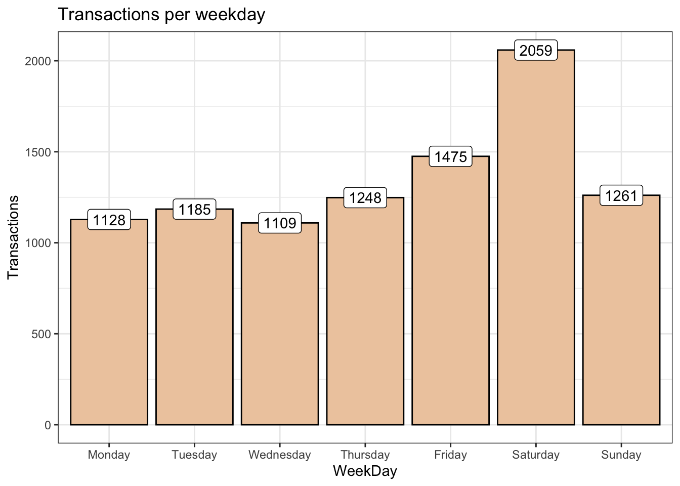
We can visualise transactions per weekday with the following code:
# Visualisation - Transactions per weekday
trans_csv %>%
  mutate(WeekDay=as.factor(weekdays(as.Date(Date)))) %>% #date converted to weekdays
  group_by(WeekDay) %>%
  summarise(Transactions=n_distinct(Transaction)) %>%
  ggplot(aes(x=WeekDay, y=Transactions)) +
  geom_bar(stat="identity", fill="peachpuff2",
           show.legend=FALSE, colour="black") +
  geom_label(aes(label=Transactions)) +
  labs(title="Transactions per weekday") +
  scale_x_discrete(limits=c("Monday", "Tuesday", "Wednesday", "Thursday",
                            "Friday", "Saturday", "Sunday")) +
theme_bw() 
The largest number of transactions occurred on Saturday (2059 transactions). This information could help the manager of the business to optimise staff time while attending to customers.
We are now ready to read the data into R as a transaction file. The arules package contains a function read.transactions to do this.
trans <- read.transactions("BreadBasket_DMS1.csv",format="single", cols=c(3,4),
                           sep=",", rm.duplicates=TRUE)
Notice that we specified cols = c(3,4). This means that column 3 of the data set is the transactionID and column 4 is the productID. cols must be a numeric and character is only allowed for header = TRUE as follows. The option rm.duplicates=TRUE removes the duplicated items from the transactions. To learn more about the read.transactions() function, please refer to the link read.transactions.
We can use summary() to summarise the data
summary(trans)## transactions as itemMatrix in sparse format with
## 9466 rows (elements/itemsets/transactions) and
## 95 columns (items) and a density of 0.0210037
##
## most frequent items:
## Coffee Bread Tea Cake Pastry (Other)
## 4528 3097 1350 983 815 8115
##
## element (itemset/transaction) length distribution:
## sizes
## 1 2 3 4 5 6 7 8 9 10
## 3949 3059 1471 662 234 64 17 4 5 1
##
## Min. 1st Qu. Median Mean 3rd Qu. Max.
## 1.000 1.000 2.000 1.995 3.000 10.000
##
## includes extended item information - examples:
## labels
## 1 Adjustment
## 2 Afternoon with the baker
## 3 Alfajores
##
## includes extended transaction information - examples:
## transactionID
## 1 1
## 2 10
## 3 100
The result shows that there are 9466 transactions (rows) and 95 items (columns). Coffee is the most frequent item and it was bought in 4528 transactions. The element (itemset/transaction) length distribution shows the size of each transactions. There exist 3949 transactions where only one item (e.g. Pastry only) was bought, while only 1 transaction include 10 items. On average, each itemset or basket contains around 2 items. The density of 0.0210037 implies that the percentage of non-zero density cells in the data matrix is about 2%.
One of the basic visualisation is the item frequency plot. For our data, we can make an absolute item frequency plot as follows:
# Absolute Item Frequency Plot
itemFrequencyPlot(trans, topN=15, type="absolute", col="wheat2",xlab="Item name",
                  ylab="Frequency (absolute)", main="Absolute Item Frequency Plot")
Indeed, coffee and bread are very frequent. Note that this does not necessarily imply that they are often bought together.
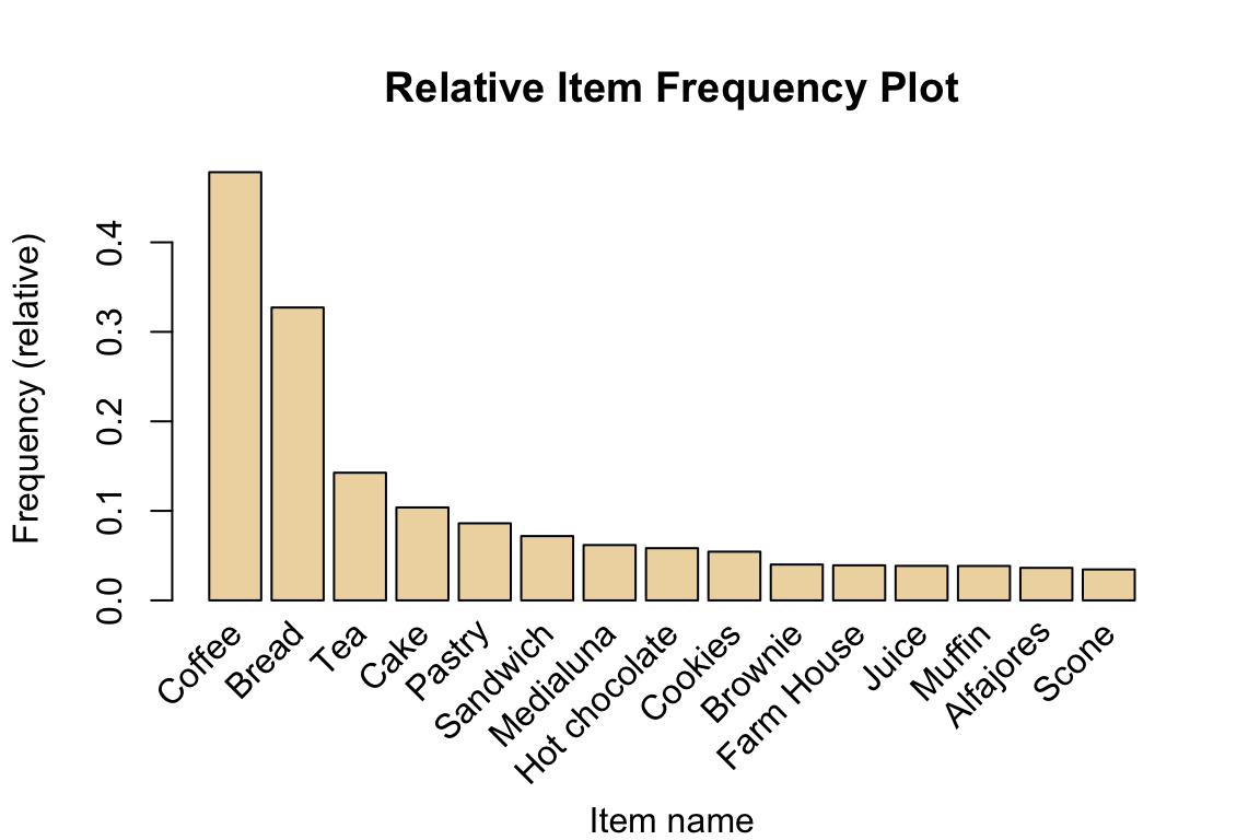
In addition to the absolute plot, a relative plot can also be obtained as follows:
# Absolute Item Frequency Plot
itemFrequencyPlot(trans, topN=15, type="relative", col="wheat2",xlab="Item name",
                  ylab="Frequency (relative)", main="Relative Item Frequency Plot")
Relative frequency plot shows how many times the items have appeared as compared to others. In principle, this is the support (defined as supp in the lecture slides). Coffee has the highest support as it is the most frequently occurring items in the absolute frequency plot.
In the grocery data example that we used as classroom/lab-lecture example, we plucked the minimum support and minimum confidence out of thin air by choosing 0.01 and 0.25, respectively, in the apriori algorithm. These values are not cast in stone. We do not want to make the choice of these values to be too low or too high. What if we try various combinations of these values simultaneously to determine the type of rule we are happy to entertain in our model? Indeed, we can do this and also examine graphically how many rules are generated for each combination before making our choice.
# Support and confidence values
supportLevels <- c(0.1, 0.05, 0.01, 0.005)
confidenceLevels <- c(0.9, 0.8, 0.7, 0.6, 0.5, 0.4, 0.3, 0.2, 0.1)

# Empty integers
rules_sup10 <- integer(length=9)
rules_sup5 <- integer(length=9)
rules_sup1 <- integer(length=9)
rules_sup0.5 <- integer(length=9)

# Apriori algorithm with a support level of 10%
for (i in 1:length(confidenceLevels)) {
  rules_sup10[i] <- length(apriori(trans, parameter=list(sup=supportLevels[1],
                                   conf=confidenceLevels[i], target="rules")))
  }

# Apriori algorithm with a support level of 5%
for (i in 1:length(confidenceLevels)){
  rules_sup5[i] <- length(apriori(trans, parameter=list(sup=supportLevels[2],
                                  conf=confidenceLevels[i], target="rules")))
  }

# Apriori algorithm with a support level of 1%
for (i in 1:length(confidenceLevels)){
  rules_sup1[i] <- length(apriori(trans, parameter=list(sup=supportLevels[3],
                                  conf=confidenceLevels[i], target="rules")))
  }

# Apriori algorithm with a support level of 0.5%
for (i in 1:length(confidenceLevels)){
  rules_sup0.5[i] <- length(apriori(trans, parameter=list(sup=supportLevels[4],
                                    conf=confidenceLevels[i], target="rules")))
  }
# Data frame
num_rules <- data.frame(rules_sup10, rules_sup5, rules_sup1, rules_sup0.5, confidenceLevels)
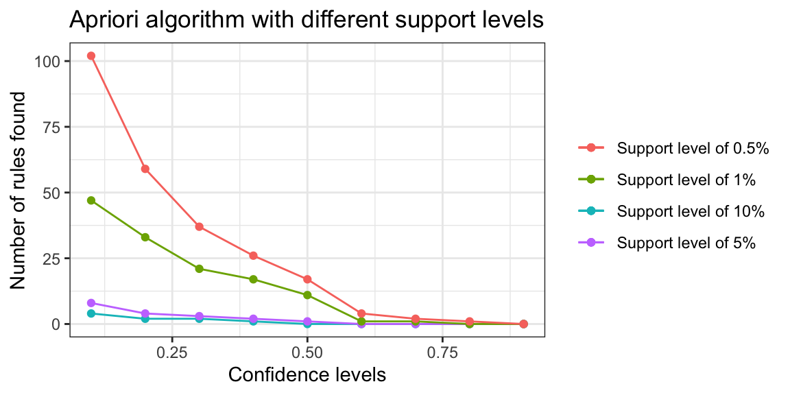
The following code is used to plot the support and confidence levels with corresponding number of rules.
# Number of rules found with a support level of 10%, 5%, 1% and 0.5%
ggplot(data=num_rules, aes(x=confidenceLevels)) +

  # Plot line and points (support level of 10%)
  geom_line(aes(y=rules_sup10, colour="Support level of 10%")) +
  geom_point(aes(y=rules_sup10, colour="Support level of 10%")) +

  # Plot line and points (support level of 5%)
  geom_line(aes(y=rules_sup5, colour="Support level of 5%")) +
  geom_point(aes(y=rules_sup5, colour="Support level of 5%")) +

  # Plot line and points (support level of 1%)
  geom_line(aes(y=rules_sup1, colour="Support level of 1%")) +
  geom_point(aes(y=rules_sup1, colour="Support level of 1%")) +

  # Plot line and points (support level of 0.5%)
  geom_line(aes(y=rules_sup0.5, colour="Support level of 0.5%")) +
  geom_point(aes(y=rules_sup0.5, colour="Support level of 0.5%")) +

  # Labs and theme
  labs(x="Confidence levels", y="Number of rules found",
       title="Apriori algorithm with different support levels") +
  theme_bw() +
  theme(legend.title=element_blank())
We can analyse the graph in order to obtain reasonable combination of support and confidence.
Support level of 10%: We only identify a few rules with very low confidence levels. This means that there are no relatively frequent associations in our data set. We can’t choose this value, the resulting rules are unrepresentative.
Support level of 5%: We only identify a rule with a confidence of at least 50%. It seems that we have to look for support levels below 5% to obtain a greater number of rules with a reasonable confidence.
Support level of 1%: We started to get dozens of rules, of which 11 rules have a confidence of at least 50%.
Support level of 0.5%. Too many rules to analyse.
To sum up, we are going to use a support level of 1% and a confidence level of 50%.
Now let’s fit the model with a support level of 1% and a confidence level of 50%. With this we obtain 11 rules.
# Apriori algorithm execution with a support level of 1% and a confidence level of 50%
rules_sup1_conf50 <- apriori(trans, parameter=list(supp=0.01,
                             conf=0.5, target="rules",minlen=2))
## Apriori
##
## Parameter specification:
## confidence minval smax arem aval originalSupport maxtime support minlen
## 0.5 0.1 1 none FALSE TRUE 5 0.01 2
## maxlen target ext
## 10 rules TRUE
##
## Algorithmic control:
## filter tree heap memopt load sort verbose
## 0.1 TRUE TRUE FALSE TRUE 2 TRUE
##
## Absolute minimum support count: 94
##
## set item appearances ...[0 item(s)] done [0.00s].
## set transactions ...[95 item(s), 9466 transaction(s)] done [0.00s].
## sorting and recoding items ... [30 item(s)] done [0.00s].
## creating transaction tree ... done [0.00s].
## checking subsets of size 1 2 3 done [0.00s].
## writing ... [11 rule(s)] done [0.00s].
## creating S4 object ... done [0.00s].
The result showed that 11 rules have been written for our analysis. The rules can be summarised using summary(rules_sup1_conf50). We can do the following to inspect the first five rules:
#Inspect association rules
inspect(rules_sup1_conf50[1:5,])
## lhs rhs support confidence coverage lift
## [1] {Spanish Brunch} => {Coffee} 0.01088105 0.5988372 0.01817029 1.251898
## [2] {Toast} => {Coffee} 0.02366364 0.7044025 0.03359392 1.472587
## [3] {Scone} => {Coffee} 0.01806465 0.5229358 0.03454469 1.093222
## [4] {Alfajores} => {Coffee} 0.01964927 0.5406977 0.03634059 1.130354
## [5] {Juice} => {Coffee} 0.02060004 0.5342466 0.03855905 1.116868
## count
## [1] 103
## [2] 224
## [3] 171
## [4] 186
## [5] 195If someone buys Spanish Brunch, they are 59.88% likely to buy Coffee too.
We can also create an HTML table widget using the inspectDT() function from the `aruslesViz package. Rules can be interactively filtered and sorted. Try the code below.
inspectDT(rules_sup1_conf50)
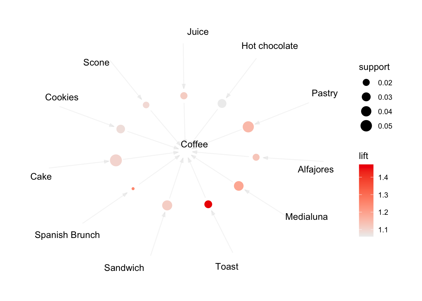
There are various plots that can be used to visualise the rules. Here is one of them:
# Graph (default layout)
plot(rules_sup1_conf50, method="graph")
Items are the labeled vertices, and rules represented as vertices connected to items using arrows.
Now consider minimum support and confidence of 0.5% and 12.5%. We can fit the model as
rules_sup05_con0125 <- apriori(trans, parameter=list(supp=0.005,
                            conf=0.125, minlen=2, target="rules"))
## Apriori
##
## Parameter specification:
## confidence minval smax arem aval originalSupport maxtime support minlen
## 0.125 0.1 1 none FALSE TRUE 5 0.005 2
## maxlen target ext
## 10 rules TRUE
##
## Algorithmic control:
## filter tree heap memopt load sort verbose
## 0.1 TRUE TRUE FALSE TRUE 2 TRUE
##
## Absolute minimum support count: 47
##
## set item appearances ...[0 item(s)] done [0.00s].
## set transactions ...[95 item(s), 9466 transaction(s)] done [0.00s].
## sorting and recoding items ... [37 item(s)] done [0.00s].
## creating transaction tree ... done [0.00s].
## checking subsets of size 1 2 3 done [0.00s].
## writing ... [86 rule(s)] done [0.00s].
## creating S4 object ... done [0.00s].
Based on this new combination of support and confidence, we have 86 rules generated. Suppose that we want to know what items customers are likely to buy given that they have purchased {Sandwich}. We can use the subset() function to obtain the subrule.
Sandwich_lhs <- subset(rules_sup05_con0125, subset = lhs %ain% c("Sandwich"))
inspect(Sandwich_lhs)
## lhs rhs support confidence coverage lift
## [1] {Sandwich} => {Tea} 0.014367209 0.2000000 0.07183604 1.4023704
## [2] {Sandwich} => {Bread} 0.017008240 0.2367647 0.07183604 0.7236728
## [3] {Sandwich} => {Coffee} 0.038242130 0.5323529 0.07183604 1.1129092
## [4] {Sandwich, Tea} => {Coffee} 0.005387703 0.3750000 0.01436721 0.7839554
## [5] {Coffee, Sandwich} => {Tea} 0.005387703 0.1408840 0.03824213 0.9878576
## [6] {Bread, Sandwich} => {Coffee} 0.007183604 0.4223602 0.01700824 0.8829642
## [7] {Coffee, Sandwich} => {Bread} 0.007183604 0.1878453 0.03824213 0.5741504
## count
## [1] 136
## [2] 161
## [3] 362
## [4] 51
## [5] 51
## [6] 68
## [7] 68
We may also want to check what items are on lhs when bread is on rhs. Suppose we want to extract the first five rules only that satisfies this sorted by confidence in decreasing order.
bread_right <- subset(rules_sup05_con0125, subset = rhs %ain% "Bread")
inspect(sort(bread_right, by="confidence", decreasing =T)[1:5])
## lhs rhs support confidence coverage lift count
## [1] {Pastry} => {Bread} 0.02915698 0.3386503 0.08609761 1.0350868 276
## [2] {Jam} => {Bread} 0.00507078 0.3380282 0.01500106 1.0331852 48
## [3] {Alfajores} => {Bread} 0.01035284 0.2848837 0.03634059 0.8707489 98
## [4] {Medialuna} => {Bread} 0.01690260 0.2735043 0.06180013 0.8359675 160
## [5] {Brownie} => {Bread} 0.01077541 0.2691293 0.04003803 0.8225954 102
As can be found below, different results are obtained when the same condition (bread) is given on lhs.
bread_left <- subset(rules_sup05_con0125, subset = lhs %ain% "Bread")
inspect(sort(bread_left, by="confidence", decreasing =T)[1:5])
## lhs rhs support confidence coverage
## [1] {Bread, Hot chocolate} => {Coffee} 0.006127192 0.4566929 0.01341644
## [2] {Bread, Cake} => {Coffee} 0.010035918 0.4298643 0.02334671
## [3] {Bread, Sandwich} => {Coffee} 0.007183604 0.4223602 0.01700824
## [4] {Bread, Medialuna} => {Coffee} 0.006761040 0.4000000 0.01690260
## [5] {Bread, Pastry} => {Coffee} 0.011197972 0.3840580 0.02915698
## lift count
## [1] 0.9547383 58
## [2] 0.8986517 95
## [3] 0.8829642 68
## [4] 0.8362191 64
## [5] 0.8028915 106
We now check if there is any redundant rules to remove them.
# redundant rules
redundant_rules <- is.redundant(rules_sup05_con0125)
summary(redundant_rules)
## Mode FALSE TRUE
## logical 68 18The number of TRUE results indicate the number of redundant rules. There are 18 of such rules in this case and the below shows the first five.
# select redundant rules and inspect the first five of them
redundant_rulesss <- rules_sup05_con0125[redundant_rules]
inspect(redundant_rulesss[1:5])
## lhs rhs support confidence coverage
## [1] {Bread, Cookies} => {Coffee} 0.005282062 0.3649635 0.01447285
## [2] {Coffee, Cookies} => {Bread} 0.005282062 0.1872659 0.02820621
## [3] {Bread, Medialuna} => {Coffee} 0.006761040 0.4000000 0.01690260
## [4] {Coffee, Medialuna} => {Bread} 0.006761040 0.1921922 0.03517853
## [5] {Bread, Hot chocolate} => {Coffee} 0.006127192 0.4566929 0.01341644
## lift count
## [1] 0.7629736 50
## [2] 0.5723795 50
## [3] 0.8362191 64
## [4] 0.5874366 64
## [5] 0.9547383 58After identifying these redundant rules and we now remove them as follows:
#By Removing the redundant rules, we are left with 68 rules
rules.set_n <- rules_sup05_con0125[!redundant_rules]
rules.set_n
## set of 68 rules