Lab 6: Market Basket Analysis
In this session, we will continue to explore the ‘BreadBasket’ data and ‘grocery’ data introduced in the lecture. Then we also perform the market basket analysis with a new dataset.
Exercise 1
Recall the following code that was used to visualize transactions per weekday in the tutorials above.
Let’s load the following packages first:
library(arules)
library(arulesViz)
library(tidyverse) # for data wrangling
library(lubridate) # work with dates and times
Remember that ‘BreadBasket_DMS1.csv’ is the updated one from the original data ‘BreadBasket_DMS.csv’ by removing NAs.
trans_csv <- read.csv('BreadBasket_DMS.csv', sep=",")

trans_csv <- trans_csv[trans_csv$Item!="NONE",]
dim(trans_csv)
## [1] 20507 4length(unique(trans_csv$Item))## [1] 94### Run the below commented lines to generate 'BreadBasket_DMS1.csv'
# write.csv(trans_csv, "BreadBasket_DMS1.csv", row.names=F)
# trans <- read.transactions("BreadBasket_DMS1.csv", format="single", cols=c(3,4),
# sep=",", rm.duplicates=TRUE)We can visualise transactions per weekday with the following code:
# Visualization - Transactions per weekday
trans_csv %>%
  mutate(WeekDay=as.factor(weekdays(as.Date(Date)))) %>% #date converted to weekdays
  group_by(WeekDay) %>%
  summarise(Transactions=n_distinct(Transaction)) %>%
  ggplot(aes(x=WeekDay, y=Transactions)) +
  geom_bar(stat="identity", fill="peachpuff2",
           show.legend=FALSE, colour="black") +
  geom_label(aes(label=Transactions)) +
  labs(title="Transactions per weekday") +
  scale_x_discrete(limits=c("Monday", "Tuesday", "Wednesday", "Thursday",
                            "Friday", "Saturday", "Sunday")) +
theme_bw() 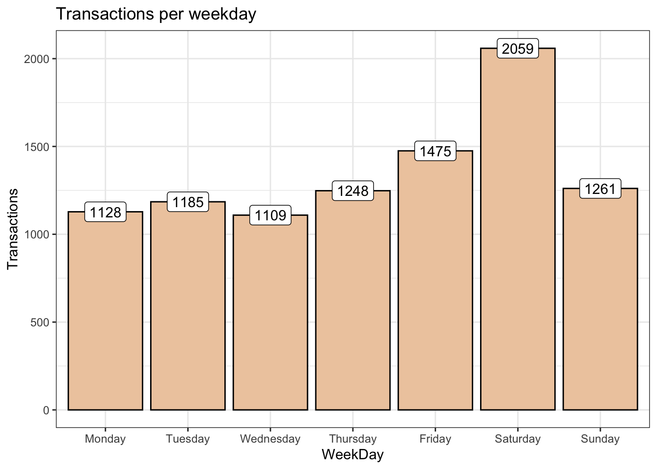
Task 1
The store manager is interested in knowing the month and the hour when sales is highest so that they can deploy staff to optimise marketing strategies, boost sales and improve customer experience. Modify the code above to visualize transactions per month and per hour, and comment on your observation.
Click for solution
# Visualization - Transactions per month
trans_csv %>%
  mutate(Month=as.factor(month(Date))) %>% #converts dates to months
  group_by(Month) %>%
  summarise(Transactions=n_distinct(Transaction)) %>%
  ggplot(aes(x=Month, y=Transactions)) +
  geom_bar(stat="identity", fill="mistyrose2",
           show.legend=FALSE, colour="black") +
  geom_label(aes(label=Transactions)) +
  labs(title="Transactions per month") +
theme_bw() 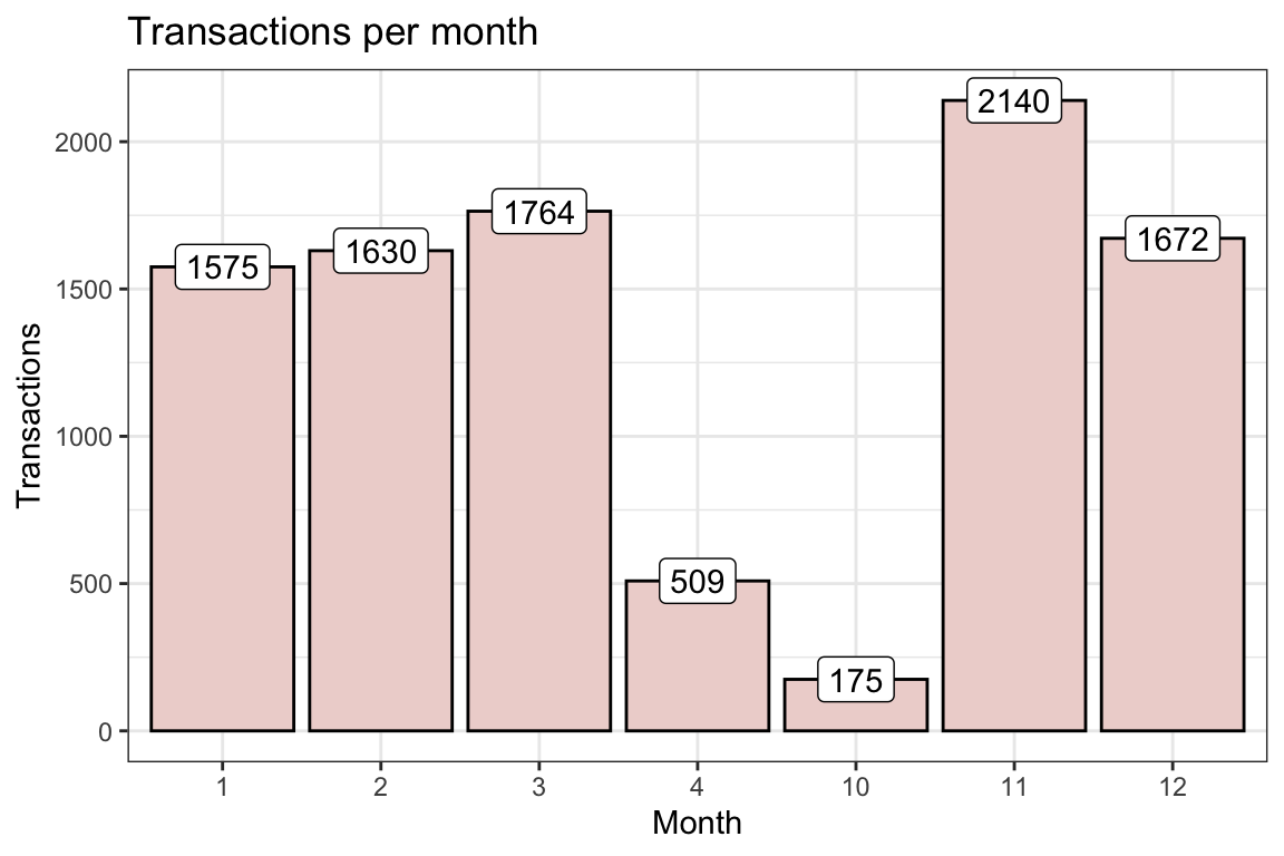
Majority of the transactions (2140) took place in November whereas 175 transactions took place in October (the least for the year).
# Visualization - Transactions per hour
trans_csv %>%
mutate(Hour=as.factor(hour(hms(Time)))) %>%
group_by(Hour) %>%
summarise(Transactions=n_distinct(Transaction)) %>%
ggplot(aes(x=Hour, y=Transactions)) +
geom_bar(stat="identity", fill="steelblue1", show.legend=FALSE, colour="black") +
geom_label(aes(label=Transactions)) +
labs(title="Transactions per hour") +
theme_bw()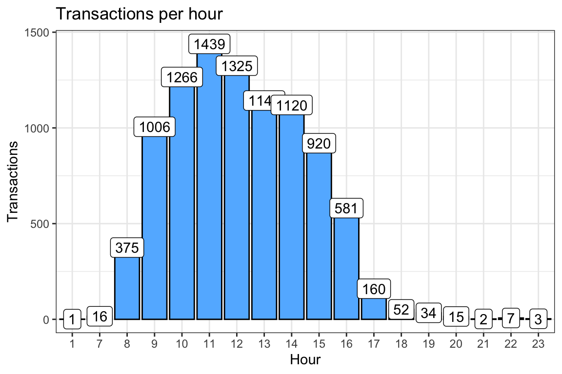 Majority of the transactions (1439) took place at 11am in the morning.
Exercise 2
We have used the apriori algorithm in the lecture to analyse the ‘Grocery data’ (data is inbuilt in the arules package), where we supplied the support and confidence that is required to generate the association rules. The result shows that there are 9835 transactions (rows) and 169 items (columns).
The task in this exercise requires you to reproduce the results in the table below without using the apriori function in arules package.
| lhs | rhs | support | confidence | coverage | lift | count |
|---|---|---|---|---|---|---|
| citrus fruit,root vegetables | other vegetables | 0.010 | 0.59 | 0.018 | 3.0 | 102 |
| tropical fruit,root vegetables | other vegetables | 0.012 | 0.58 | 0.021 | 3.0 | 121 . |
These results are taken from the lecture note.
In the exercise, you are required to read the Groceries data into R using readLines() function. It is advisable that you load the data from the groceries.csv file on Blackboard or directly from the internet as follows:
grocery.text <- readLines("https://github.com/stedy/Machine-Learning-with-R-datasets/blob/master/groceries.csv")
Task 2a
Compute the 1) support, 2) coverage, 3) confidence and 4) lift for the rule: {citrus fruit, root vegetables} \(\Rightarrow\) {other vegetables}.
*Hint: To be able to count the number of times a transaction occur in a database, you will need a function to detect string variable. This can be obtained from the stringr package. To help you to understand, a string is a sequence of characters and we represent strings using double (e.g. “Hello”) or single (e.g. ‘Hello’) quotes in R.
Consider a scenario where we are interested in the number of times item {A} alone and items {A, B} appear in a database. You can use the following syntax to count the number of transactions for each case:*
library(stringr)

sum(str_detect(grocery.text, "A"))
## [1] 84sum(str_detect(grocery.text, "A") & str_detect(grocery.text, "B"))## [1] 14
Click for solution
library(stringr)
#{citrus fruit,root vegetables} => {other vegetables}
######## Support
a_supp = sum((str_detect(grocery.text, "citrus fruit") &
str_detect(grocery.text, "root vegetables")) &
str_detect(grocery.text, "other vegetables"))
a_supp## [1] 102a_supp/9835## [1] 0.01037112######## Coverage: support for the antecedent
a_cov = sum((str_detect(grocery.text, "citrus fruit") & str_detect(grocery.text, "root vegetables")))
a_cov## [1] 174a_cov/9835## [1] 0.01769192######## Confidence
# The confidence that shopper who bought citrus fruit & root vegetables will buy other vegetables is
a_conf = a_supp/a_cov
a_conf## [1] 0.5862069######## Lift- the ratio between X and Y together and X and Y independently.
# We need support of X and Y = a_supp; support of X = a_cov and support of Y
y_supp = sum(str_detect(grocery.text, "other vegetables"))/9835
a_lift = a_supp/(a_cov * y_supp)
a_lift## [1] 3.029608
Task 2b
Similarly, compute the 1) support, 2) coverage, 3) confidence and 4) lift for the rule: {tropical fruit,root vegetables} \(\Rightarrow\) {other vegetables}.
Click for solution
######## Support
b_supp = sum((str_detect(grocery.text, "tropical fruit") &
                str_detect(grocery.text, "root vegetables")) &
               str_detect(grocery.text, "other vegetables"))
b_supp
## [1] 121b_supp/9835## [1] 0.012303######## Coverage: support for the antecedent
b_cov = sum((str_detect(grocery.text, "tropical fruit") & str_detect(grocery.text, "root vegetables")))
b_cov## [1] 207b_cov/9835## [1] 0.02104728######## Confidence
# The confidence that shopper who bought tropical fruit & root vegetables will buy other vegetables is
b_conf = b_supp/b_cov
b_conf## [1] 0.5845411######## Lift
by_supp = sum(str_detect(grocery.text, "other vegetables"))/9835
b_lift = b_supp/(b_cov * by_supp)
b_lift## [1] 3.020999
Exercise 3
Consider the Market Basket Optimisation data set, which is publicly available HERE. The data set contains 7501 transaction records where every record consists of the list of items sold in just one transaction.
Task 3a
Determine the correct way of reading this data into R using read.transactions(). A copy of the data Market_Basket_Optimisation.csv can be downloaded from Blackboard.
Click for solution
The key part of this task is to use format = “basket”. We use this format when each line in the transaction data file represents a transaction where the items (item labels) are separated by the characters specified by sep.
trans <- read.transactions('Market_Basket_Optimisation.csv', format="basket",
                           sep=",", rm.duplicates=TRUE)
## distribution of transactions with duplicates:
## 1
## 5summary(trans)## transactions as itemMatrix in sparse format with
## 7501 rows (elements/itemsets/transactions) and
## 119 columns (items) and a density of 0.03288973
##
## most frequent items:
## mineral water eggs spaghetti french fries chocolate
## 1788 1348 1306 1282 1229
## (Other)
## 22405
##
## element (itemset/transaction) length distribution:
## sizes
## 1 2 3 4 5 6 7 8 9 10 11 12 13 14 15 16
## 1754 1358 1044 816 667 493 391 324 259 139 102 67 40 22 17 4
## 18 19 20
## 1 2 1
##
## Min. 1st Qu. Median Mean 3rd Qu. Max.
## 1.000 2.000 3.000 3.914 5.000 20.000
##
## includes extended item information - examples:
## labels
## 1 almonds
## 2 antioxydant juice
## 3 asparagusThe first five transactions can be obtained via the code below.
items <- readLines('Market_Basket_Optimisation.csv', n=5)
items
## [1] "shrimp,almonds,avocado,vegetables mix,green grapes,whole weat flour,yams,cottage cheese,energy drink,tomato juice,low fat yogurt,green tea,honey,salad,mineral water,salmon,antioxydant juice,frozen smoothie,spinach,olive oil"
## [2] "burgers,meatballs,eggs"
## [3] "chutney"
## [4] "turkey,avocado"
## [5] "mineral water,milk,energy bar,whole wheat rice,green tea"Here we will follow the analysis done in Workshop: MBA but with a different data. We will find the best combination of support and confidence to uncover reasonable rules. Also we will identify redundant rules, if any.
Task 3b
Find the item that is the most frequently bought.
Click for solution
# Absolute Item Frequency Plot
itemFrequencyPlot(trans, topN=15, type="absolute", col = "wheat2", xlab="Item name",
                  ylab="Frequency (absolute)", main="Absolute Item Frequency Plot")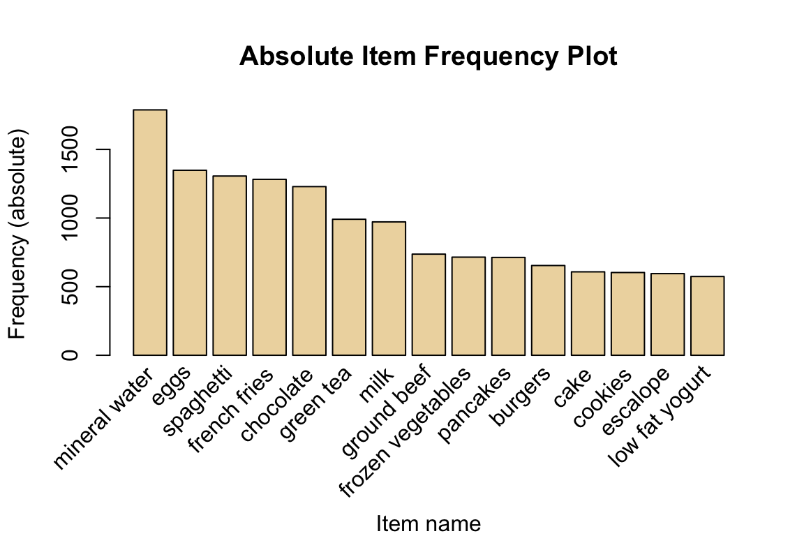
Task 3c
Now we are going to try various combinations of support and confidence values simultaneously to determine the type of rule we are happy to entertain in our model.
# Support and confidence values
supportLevels <- c(0.1, 0.05, 0.01, 0.005)
confidenceLevels <- seq(0.9, 0.1, by=-0.05)
Revisit the R code used in Workshop: MBA and choose the appropriate combination of support and confidence levels.
Click for solution
# Empty integers
rules_sup10 <- integer(length=9)
rules_sup5 <- integer(length=9)
rules_sup1 <- integer(length=9)
rules_sup0.5 <- integer(length=9)

# Apriori algorithm with a support level of 10%
for (i in 1:length(confidenceLevels)) {

  rules_sup10[i] <- length(apriori(trans, parameter=list(sup=supportLevels[1],
                                                         conf=confidenceLevels[i], target="rules")))
}

# Apriori algorithm with a support level of 5%
for (i in 1:length(confidenceLevels)){

  rules_sup5[i] <- length(apriori(trans, parameter=list(sup=supportLevels[2],
                                                        conf=confidenceLevels[i], target="rules")))
}

# Apriori algorithm with a support level of 1%
for (i in 1:length(confidenceLevels)){

  rules_sup1[i] <- length(apriori(trans, parameter=list(sup=supportLevels[3],
                                                        conf=confidenceLevels[i], target="rules")))
}

# Apriori algorithm with a support level of 0.5%
for (i in 1:length(confidenceLevels)){

  rules_sup0.5[i] <- length(apriori(trans, parameter=list(sup=supportLevels[4],
                                                          conf=confidenceLevels[i], target="rules")))
}
# Data frame
num_rules <- data.frame(rules_sup10, rules_sup5, rules_sup1, rules_sup0.5, confidenceLevels)
num_rules## rules_sup10 rules_sup5 rules_sup1 rules_sup0.5 confidenceLevels
## 1 0 0 0 0 0.90
## 2 0 0 0 0 0.85
## 3 0 0 0 0 0.80
## 4 0 0 0 0 0.75
## 5 0 0 0 0 0.70
## 6 0 0 0 0 0.65
## 7 0 0 0 1 0.60
## 8 0 0 0 5 0.55
## 9 0 0 2 20 0.50
## 10 0 0 6 41 0.45
## 11 0 0 18 91 0.40
## 12 0 0 31 148 0.35
## 13 0 2 63 261 0.30
## 14 0 4 95 395 0.25
## 15 1 7 164 599 0.20
## 16 5 11 232 802 0.15
## 17 7 13 316 1066 0.10
# Number of rules found with a support level of 10%, 5%, 1% and 0.5%
ggplot(data=num_rules, aes(x=confidenceLevels)) +

  # Plot line and points (support level of 10%)
  geom_line(aes(y=rules_sup10, colour="Support level of 10%")) +
  geom_point(aes(y=rules_sup10, colour="Support level of 10%")) +

  # Plot line and points (support level of 5%)
  geom_line(aes(y=rules_sup5, colour="Support level of 5%")) +
  geom_point(aes(y=rules_sup5, colour="Support level of 5%")) +

  # Plot line and points (support level of 1%)
  geom_line(aes(y=rules_sup1, colour="Support level of 1%")) +
  geom_point(aes(y=rules_sup1, colour="Support level of 1%")) +

  # Plot line and points (support level of 0.5%)
  geom_line(aes(y=rules_sup0.5, colour="Support level of 0.5%")) +
  geom_point(aes(y=rules_sup0.5, colour="Support level of 0.5%")) +

  # Labs and theme
  labs(x="Confidence levels", y="Number of rules found",
       title="Apriori algorithm with different support levels") +
  theme_bw() +
  theme(legend.title=element_blank())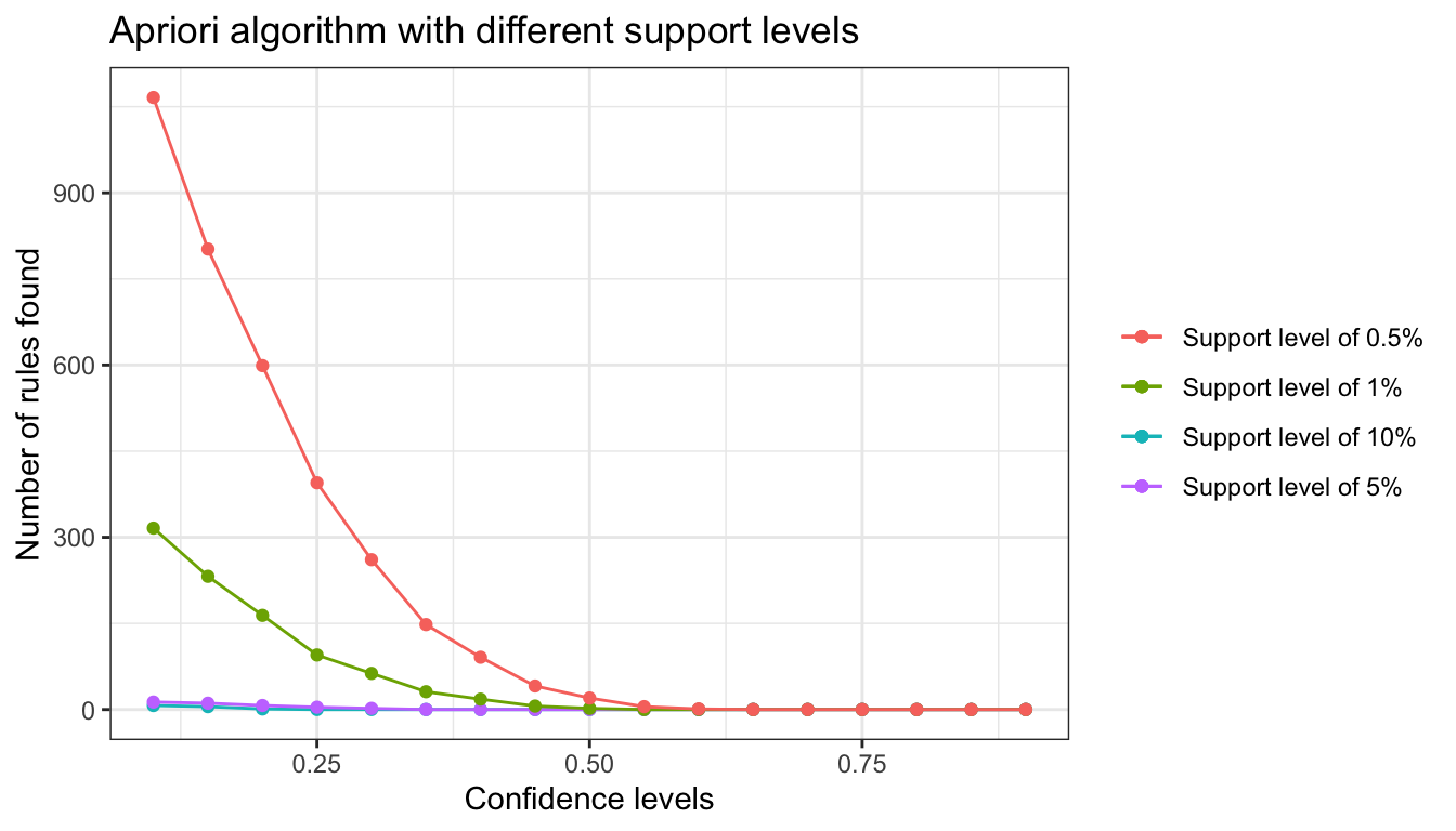
Here we might choose support = 0.01 and confidence = 0.25. This will generate less than 100 rules.
Task 3d
Fit the model with the chosen combination of support and confidence level then inspect the first five rules. Check if there is any redundant rules.
Click for solution
# Apriori algorithm execution with a support level of 1% and a confidence level of 25%
rules_sup1_conf25 <- apriori(trans, parameter=list(supp=0.01,
                                                   conf=0.25, minlen=2, target="rules"))
## Apriori
##
## Parameter specification:
## confidence minval smax arem aval originalSupport maxtime support minlen
## 0.25 0.1 1 none FALSE TRUE 5 0.01 2
## maxlen target ext
## 10 rules TRUE
##
## Algorithmic control:
## filter tree heap memopt load sort verbose
## 0.1 TRUE TRUE FALSE TRUE 2 TRUE
##
## Absolute minimum support count: 75
##
## set item appearances ...[0 item(s)] done [0.00s].
## set transactions ...[119 item(s), 7501 transaction(s)] done [0.00s].
## sorting and recoding items ... [75 item(s)] done [0.00s].
## creating transaction tree ... done [0.00s].
## checking subsets of size 1 2 3 4 done [0.00s].
## writing ... [95 rule(s)] done [0.00s].
## creating S4 object ... done [0.00s].rules_sup1_conf25## set of 95 rules
We now inspect the first five rules.
#Inspect association rules
inspect(rules_sup1_conf25[1:5,])
## lhs rhs support confidence coverage lift
## [1] {cereals} => {mineral water} 0.01026530 0.3989637 0.02572990 1.673729
## [2] {red wine} => {spaghetti} 0.01026530 0.3649289 0.02812958 2.095966
## [3] {red wine} => {mineral water} 0.01093188 0.3886256 0.02812958 1.630358
## [4] {avocado} => {mineral water} 0.01159845 0.3480000 0.03332889 1.459926
## [5] {fresh bread} => {mineral water} 0.01333156 0.3095975 0.04306093 1.298820
## count
## [1] 77
## [2] 77
## [3] 82
## [4] 87
## [5] 100
The following codes show that there is no redundant rule.
# redundant rules
redundant_rules25 <- is.redundant(rules_sup1_conf25)
summary(redundant_rules25)
## Mode FALSE
## logical 95