Lab 5: Hierarchical clustering and Model-based clustering
In this session, we will first explore a hybrid method called Hierarchical K-means Clustering which improved the robustness of the K-means clustering. We will also explore the model-based clustering approach.
Exercise 1 (Hierarchical K-means Clustering)
The final K-means clustering solution is sensitive to the initial random selection of cluster centers. The hkmeans() function in factoextra package provides a hybrid method for improving K-means results. The algorithm is summarised as follows:
Step 1: Compute hierarchical clustering and cut the tree into k-clusters
Step 2: Compute the centre (i.e the mean) of each cluster
Step 3: Compute k-means by using the set of cluster centers (defined in step 2) as the initial cluster centers.
Note that, k-means algorithm will improve the initial partitioning generated at Step 2 of the algorithm. We will illustrate the method using the iris data.
library(factoextra)

# Compute hierarchical k-means clustering
iris.scaled <- scale(iris[, -5])
res.hk <- hkmeans(iris.scaled, k=3, hc.metric = "euclidean", hc.method ="complete")

# Component returned by hkmeans()
res.hk
## Hierarchical K-means clustering with 3 clusters of sizes 50, 53, 47
##
## Cluster means:
## Sepal.Length Sepal.Width Petal.Length Petal.Width
## 1 -1.01119138 0.85041372 -1.3006301 -1.2507035
## 2 -0.05005221 -0.88042696 0.3465767 0.2805873
## 3 1.13217737 0.08812645 0.9928284 1.0141287
##
## Clustering vector:
## [1] 1 1 1 1 1 1 1 1 1 1 1 1 1 1 1 1 1 1 1 1 1 1 1 1 1 1 1 1 1 1 1 1 1 1 1 1 1
## [38] 1 1 1 1 1 1 1 1 1 1 1 1 1 3 3 3 2 2 2 3 2 2 2 2 2 2 2 2 3 2 2 2 2 3 2 2 2
## [75] 2 3 3 3 2 2 2 2 2 2 2 3 3 2 2 2 2 2 2 2 2 2 2 2 2 2 3 2 3 3 3 3 2 3 3 3 3
## [112] 3 3 2 2 3 3 3 3 2 3 2 3 2 3 3 2 3 3 3 3 3 3 2 2 3 3 3 2 3 3 3 2 3 3 3 2 3
## [149] 3 2
##
## Within cluster sum of squares by cluster:
## [1] 47.35062 44.08754 47.45019
## (between_SS / total_SS = 76.7 %)
##
## Available components:
##
## [1] "cluster" "centers" "totss" "withinss" "tot.withinss"
## [6] "betweenss" "size" "iter" "ifault" "data"
## [11] "hclust"A careful look at the output indicates that the object res.hk returned output is similar to the K-means model. Revisit the last workshop material (Workshop: K-means) to answer the following question.
Task 1
What is the percentage of variance explained by the three cluster means? How does this compare with the result using K-means in the workshop?
Click for solution
dd <- cbind(iris, cluster = res.hk$cluster)
table(dd$Species,dd$cluster)
##
## 1 2 3
## setosa 50 0 0
## versicolor 0 39 11
## virginica 0 14 36
Exercise 2 (Model-based clustering)
In this exercise, we will use the model-based clustering approach to analyse the USArrests data.
library(mclust)
data("USArrests")
datUS <- scale(USArrests)
Task 2a
Make sure that the most appropriate model is selected via BIC. To choose the best model among a lot of combinations of \(k\), the number of mixture components (clusters), and the models that can be chosen from the command Mclust(), we generate the array named resu in the following.
G <- c(2,3,4,5,6)
modelNames <- c("EII", "VII", "EEI", "VEI", "EVI", "VVI", "EEE", "EEV", "VEV", "VVV")

nnr <- length(G)*length(modelNames)
resu  <- array(data=NA, dim=c(nnr,3), dimnames=list(paste(1:nnr),c("G", "modelNames", "BIC")))
Create a code using for loop (for (i in G) & for(j in modelNames)) to fill the empty matrix resu.
Click for solution
counter <- 1

for (i in G){
  for(j in modelNames){
mc_option <- Mclust(datUS, G = i, modelNames = j)
  resu[counter, 1] <- as.numeric(i)
  resu[counter, 2] <- paste(j)
  resu[counter, 3] <- as.numeric(mc_option$BIC)
  if (counter < nrow(resu)) counter <- counter+1
  }
}

G <- as.numeric(resu[,1])
bic <- as.numeric(resu[,3])
model <- resu[,2]
dat <- data.frame(G, bic, model)
Task 2b
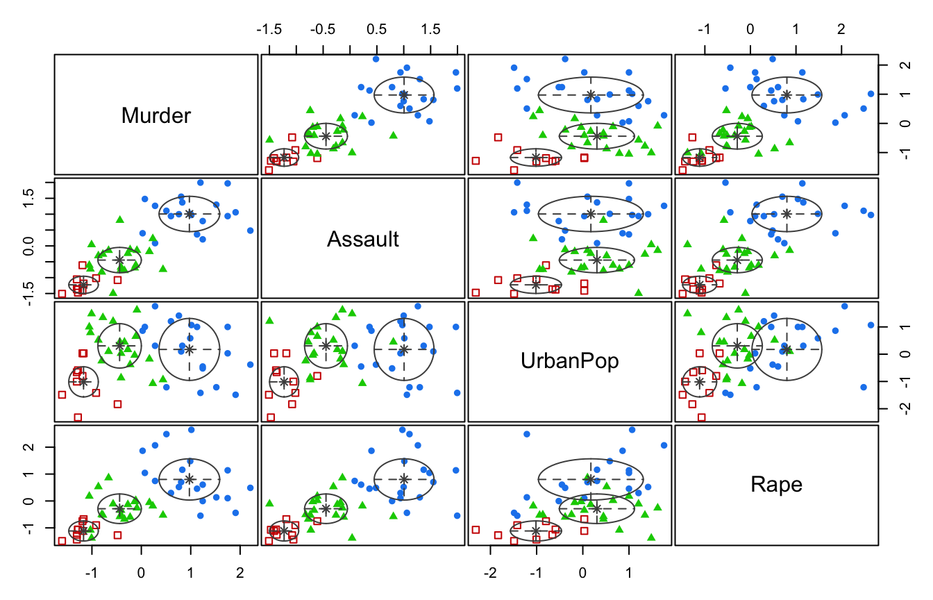
Choose the model combination which gives the largest BIC and use the selected one to fit the final model. Also visualise the results.
Click for solution
aa <- subset(dat, bic == max(bic))
aa
## G bic model
## 14 3 -512.9677 VEImcUS <- Mclust(datUS, G = 3, modelNames = "VEI") # Model-based-clustering
summary(mcUS)## ----------------------------------------------------
## Gaussian finite mixture model fitted by EM algorithm
## ----------------------------------------------------
##
## Mclust VEI (diagonal, equal shape) model with 3 components:
##
## log-likelihood n df BIC ICL
## -217.3636 50 20 -512.9677 -517.5878
##
## Clustering table:
## 1 2 3
## 20 10 20plot(mcUS, what = "classification")
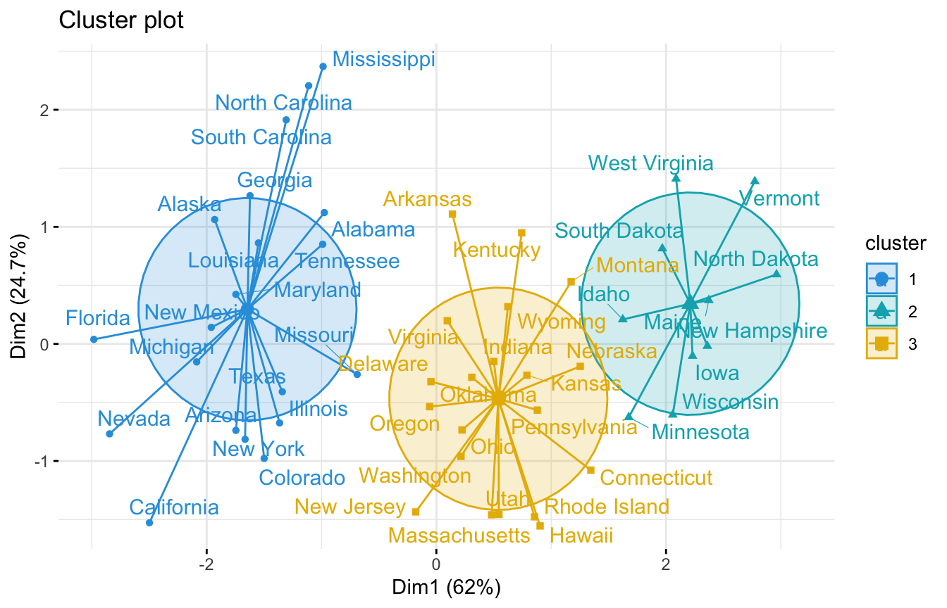
We can also use the fviz_cluster function to visualise the clusters:
library(factoextra)
fviz_cluster(mcUS, data = datUS,
             palette = c("#2E9FDF", "#00AFBB", "#E7B800"),
             ellipse.type = "euclid", # Concentration ellipse
             star.plot = TRUE, # Add segments from centroids to items
             repel = TRUE, # Avoid label overplotting (slow)
             ggtheme = theme_minimal()
)
If you find the for loop (for (i in G) & for(j in modelNames)) too complicated, you can fit the models without using modelNames for each of G = {2, 3, 4, 5 ,6} and manually look at the highest BIC value. That is:
mc_bic2 <- Mclust(datUS, G = 2)
mc_bic2$BIC
## Bayesian Information Criterion (BIC):
## EII VII EEI VEI EVI VVI EEE
## 2 -538.8433 -540.8772 -527.0649 -528.6261 -535.4764 -537.2757 -526.5854
## VEE EVE VVE EEV VEV EVV VVV
## 2 -523.2595 -526.9245 -528.7491 -525.21 -527.3192 -535.5687 -537.8664
##
## Top 3 models based on the BIC criterion:
## VEE,2 EEV,2 EEE,2
## -523.2595 -525.2100 -526.5854max(mc_bic2$BIC)## [1] -523.2595The maximum bic value here is -523.2595 using VEE
mc_bic3 <- Mclust(datUS, G = 3)
mc_bic3$BIC
## Bayesian Information Criterion (BIC):
## EII VII EEI VEI EVI VVI EEE
## 3 -537.5736 -525.7363 -526.2293 -512.9677 -543.7187 -527.7402 -532.9476
## VEE EVE VVE EEV VEV EVV VVV
## 3 -523.1587 -524.2615 -534.9031 -518.329 -540.6332 -533.7338 -537.8338
##
## Top 3 models based on the BIC criterion:
## VEI,3 EEV,3 VEE,3
## -512.9677 -518.3290 -523.1587max(mc_bic3$BIC)## [1] -512.9677The maximum bic value here is -512.9677 using VEI
mc_bic4 <- Mclust(datUS, G = 4)
mc_bic4$BIC
## Bayesian Information Criterion (BIC):
## EII VII EEI VEI EVI VVI EEE
## 4 -521.7755 -526.6926 -517.8144 -519.4226 -543.1231 -543.7167 -534.2095
## VEE EVE VVE EEV VEV EVV VVV
## 4 -532.9796 -532.6512 -541.8985 -553.6194 -567.6144 -559.0539 -585.2552
##
## Top 3 models based on the BIC criterion:
## EEI,4 VEI,4 EII,4
## -517.8144 -519.4226 -521.7755max(mc_bic4$BIC)## [1] -517.8144The maximum bic value here is -517.8144 using EEI
mc_bic5 <- Mclust(datUS, G = 5)
mc_bic5$BIC
## Bayesian Information Criterion (BIC):
## EII VII EEI VEI EVI VVI EEE
## 5 -533.2121 -538.0429 -531.1563 -534.6521 -561.6267 -564.2804 -548.5219
## VEE EVE VVE EEV VEV EVV VVV
## 5 -550.5176 -560.2447 -573.9986 -579.1599 -586.9238 -604.4145 -618.2049
##
## Top 3 models based on the BIC criterion:
## EEI,5 EII,5 VEI,5
## -531.1563 -533.2121 -534.6521max(mc_bic5$BIC)## [1] -531.1563The maximum bic value here is -531.1563 using EEI
mc_bic6 <- Mclust(datUS, G = 6)
mc_bic6$BIC
## Bayesian Information Criterion (BIC):
## EII VII EEI VEI EVI VVI EEE VEE
## 6 -550.2138 -545.536 -548.212 -550.4491 -577.6596 -595.8654 -566.1261 -564.7011
## EVE VVE EEV VEV EVV VVV
## 6 -591.5751 -590.6452 -590.6371 -600.8944 -629.884 -642.288
##
## Top 3 models based on the BIC criterion:
## VII,6 EEI,6 EII,6
## -545.5360 -548.2120 -550.2138max(mc_bic6$BIC)## [1] -545.536The maximum bic value here is -545.536 using VII.
Therefore, -512.9677 with VEI resulted in maximum BIC value and as such we will use G=3 as the optimal number of cluster. This is same as the result we obtained using the for loop above.