Lab 4: K-means clustering
Exercise 1
In this exercise, you will perform K-means clustering manually, with \(K = 2\), on a small example with \(n = 6\) observations and \(p = 2\) features. The observations are as follows:
x1 <- c(1,1,0,5,6,4)
x2 <- c(4,3,4,1,2,0)
dat <- cbind(x1,x2)
dat
## x1 x2
## [1,] 1 4
## [2,] 1 3
## [3,] 0 4
## [4,] 5 1
## [5,] 6 2
## [6,] 4 0
Task 1
The step-by-step procedure for carrying out this task can be found from the lecture note and we are trying to implement it.
Plot the observations.
Choose \(m_{1} = (1,4)\) and \(m_{2} = (5,1)\) as initial centroid.
Compute the centroid for each cluster.
Assign each observation to the centroid to which it is closest, in terms of Euclidean distance. Report the cluster labels for each observation.
Repeat (iii) and (iv) until the answers obtained stop changing.
In your plot from (i), color the observations according to the cluster labels obtained.
You can use the codes below to compute the Euclidean distance between each observation and the suggested centroids.
euclid = function(a, b) {
  return(sqrt((a[1] - b[1])^2 + (a[2]-b[2])^2))
}

mm <- function(x, centroid1){
 xx = rep(NA, nrow(x))
for (i in 1:nrow(x)) {
    xx[i]=euclid(x[i,], centroid1)
}
return(xx)
} mm(dat, c(1,4))## [1] 0.000000 1.000000 1.000000 5.000000 5.385165 5.000000mm(dat, c(5,1))## [1] 5.000000 4.472136 5.830952 0.000000 1.414214 1.414214Alternatively you can use the dist() function in R. Assign the points in the data into clusters (you may refer to this as labels). You can update the centroids with the following codes:
labels = c(1,1,1,2,2,2)
centroid1 = c(mean(dat[labels==1, 1]), mean(dat[labels==1, 2]))
centroid2 = c(mean(dat[labels==2, 1]), mean(dat[labels==2, 2]))
centroid1
## [1] 0.6666667 3.6666667centroid2## [1] 5 1This results in the updated centroids. Now repeat this method until the clusters are no longer changing.
Click for solution
# First plot
plot(dat[,1], dat[,2], xlab="x1", ylab="x2")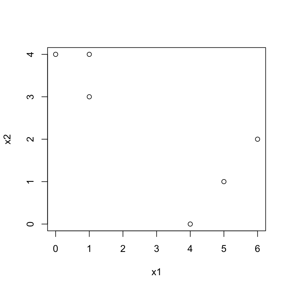
labelf = c(1,1,1,2,2,2)
centroid1f = c(mean(dat[labelf==1, 1]), mean(dat[labelf==1, 2]))
centroid2f = c(mean(dat[labelf==2, 1]), mean(dat[labelf==2, 2]))
centroid1f
## [1] 0.6666667 3.6666667centroid2f## [1] 5 1plot(dat[,1], dat[,2], col=(labelf+1), pch=20, cex=2, xlab="x1", ylab="x2")
points(centroid1f[1], centroid1f[2], col=2, pch=4)
points(centroid2f[1], centroid2f[2], col=3, pch=4)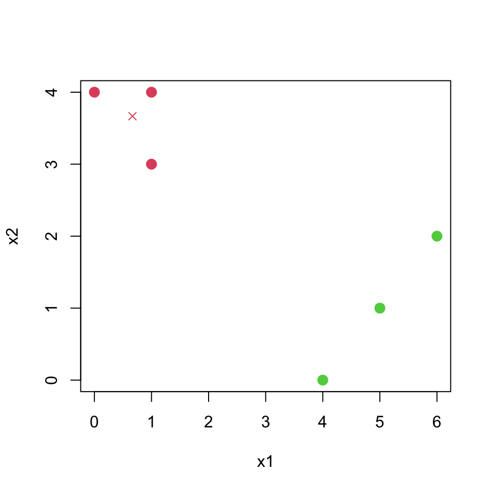
So two clusters have been identified in the end.
Exercise 2
In this exercise, we will simulate data, and then perform PCA and K-means clustering on the data.
We are required to generate a data set with 20 observations in each of three classes (i.e. 60 observations in total), and 50 variables. Read and run the code given below which will help you to start:
# Part (a) generate data:
#
K = 3  # the number of classes
n = 20 # the number of samples per class
p = 50 # the number of variables

set.seed(123)
# Create data for class 1:
X_1 = matrix( rnorm(n*p), nrow=n, ncol=p )
for( row in 1:n ){
  X_1[row,] = X_1[row,] + rep( 1, p )
}

# Create data for class 2:
X_2 = matrix( rnorm(n*p), nrow=n, ncol=p )
for( row in 1:n ){
  X_2[row,] = X_2[row,] + rep( -1, p )
}

# Create data for class 3:
X_3 = matrix( rnorm(n*p), nrow=n, ncol=p )
for( row in 1:n ){
  X_3[row,] = X_3[row,] + c( rep( 1, p/2 ), rep( -1, p/2 ) )
}

X <- rbind(X_1, X_2, X_3)
dim(X)
## [1] 60 50
Task 2a
Perform K-means clustering on the observations with \(K = 3\). How well do the clusters that you obtained in K-means clustering compare to the true class labels? Use fviz_cluster function for visualisation.
Click for solution
# Kmeans on the original data
library(factoextra)
Xs <- scale(X)

kmean.out = kmeans(Xs, centers=3, nstart=25)
fviz_cluster(kmean.out, Xs, ellipse.type = "norm")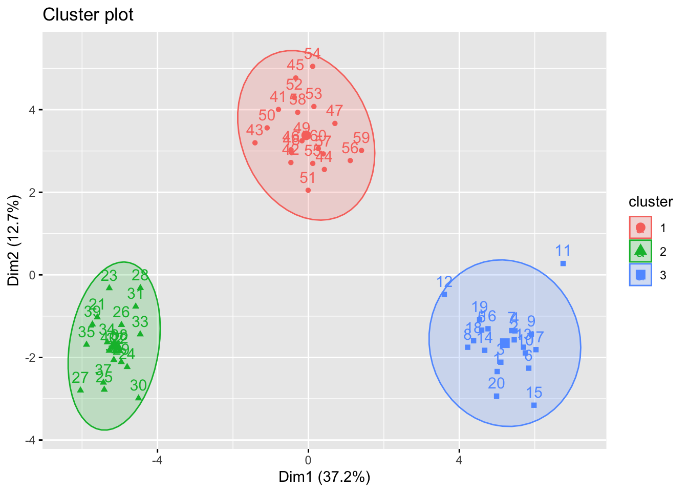
Task 2b
To check the optimal number of clusters, we perform the silhouette analysis. First run \(K\)-means clustering for different sizes of \(K = 2, 3, \ldots, 6\).
Click for solution
kmean1 = kmeans(Xs, centers=1, nstart=25)
kmean2 = kmeans(Xs, centers=2, nstart=25)
kmean3 = kmeans(Xs, centers=3, nstart=25)
kmean4 = kmeans(Xs, centers=4, nstart=25)
kmean5 = kmeans(Xs, centers=5, nstart=25)
kmean6 = kmeans(Xs, centers=6, nstart=25)
Or there is another way of doing this.
set.seed(2023)
for(i in 1:6){
  assign(paste("kmean", i, sep=""), kmeans(Xs, centers=i, nstart=25))
}
Task 2c
Now we compute the silhouette width for each clustering output and plot it to find the optimal \(K\) where the silhouette width is maximised.
Click for solution
Here we can use the for loop again.
library(cluster)
sil.width <- rep(NA, 6)
sil.width[1] <- 0

for(i in 2:6){
  kmean.out <- get(paste("kmean", i, sep=""))
  sil <- silhouette(kmean.out$cluster, dist(Xs))
  sil.width[i] <- summary(sil)$avg.width
}

plot(1:6,  sil.width, type="b", pch=19, xlab="k", ylab="silhouette width")
abline(v=which.max(sil.width), col=2, lty=2)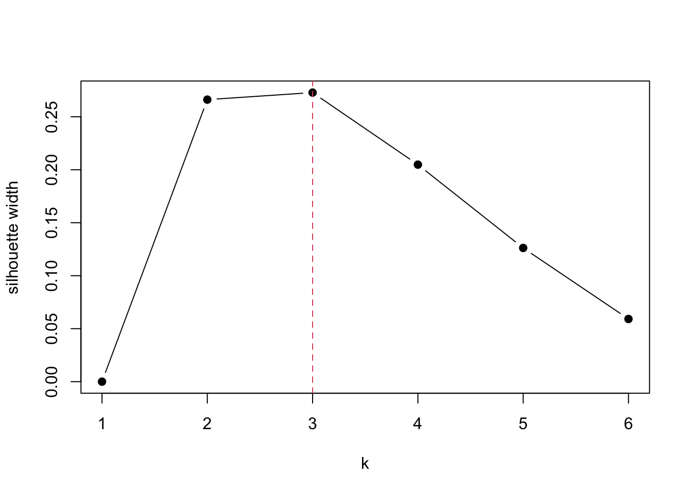
It seems that \(k=3\) is a reasonable choice. We can get the similar plot by running below.
library(mclust)
#K-means
fviz_nbclust(Xs, kmeans, method = "silhouette")+labs(title = "K-means")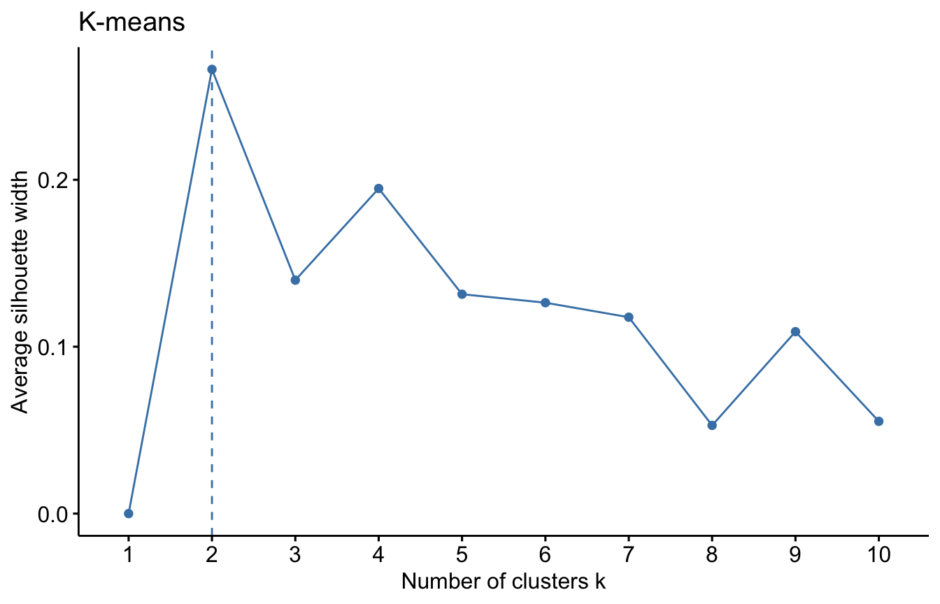
However, the silhoutte width is maximised at \(k=2\) here. Why? because the function fviz_nbclust() use the kmeans() inside but with the default inputs e.g. nstart is set to 1 and iter.max is set to 10. If we run the above code built on silhouette() function after tweaking the objects kmean1, kmean2, …, kmean6 again without set.seed() and using different nstart e.g. nstart=1, then it will give different results whenever you run the code. To get a robust result, it is important to try different initial clusters and select the best results which you can control by changing nstart option in kmeans() function.
Task 2d
Repeat the Tasks 2c and 2d with the updated data shown below (only the variables \(X_2\) and \(X_3\) are updated). Are the two optimal \(K\)s obtained as the same?
# Part (a) generate data:
#
K = 3  # the number of classes
n = 20 # the number of samples per class
p = 50 # the number of variables

# Create data for class 1:
X_1 = matrix( rnorm(n*p), nrow=n, ncol=p )
for( row in 1:n ){
  X_1[row,] = X_1[row,] + rep( 1, p )
}

# Create data for class 2:
X_2 = matrix( rnorm(n*p), nrow=n, ncol=p )
for( row in 1:n ){
  X_2[row,] = X_2[row,] + rep( -5, p )
}

# Create data for class 3:
X_3 = matrix( rnorm(n*p), nrow=n, ncol=p )
for( row in 1:n ){
  X_3[row,] = X_3[row,] + c( rep( 5, p/2 ), rep( -5, p/2 ) )
}

X <- rbind(X_1, X_2, X_3)
Xs <- scale(X)

kmean.out = kmeans(Xs, centers=3, nstart=25)
fviz_cluster(kmean.out, Xs, ellipse.type = "norm")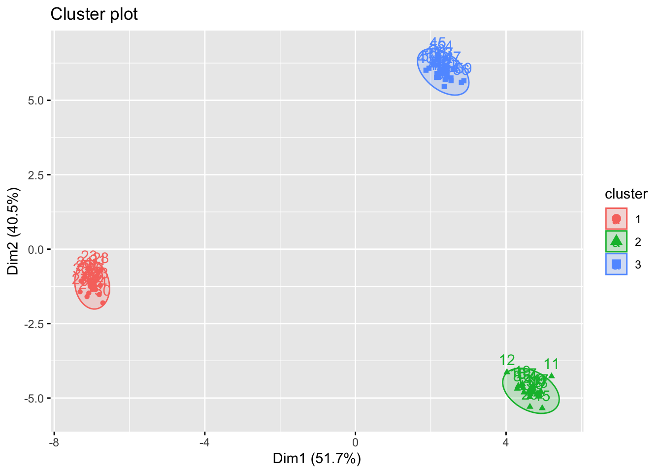
Click for solution
It is highly likely that the optimal \(K\)s are obtained as the same due to stronger signal (i.e. clusters are more clearly detected even by eyes).