Lab 1: Introduction
In this introduction session, we are going to review some basic mathematics which will be useful in the rest of this module. In exercise 1, we will look at an example of multivariate data and in exercise 2, we will explore how we can measure the distance between two observations. In exercises 3 and 4, we will go through eigendecomposition and singular value decomposition.
Exercise 1 (Multivariate normal distribution)
We have \(n\) observations and \(p\) features (variables) with a given data matrix of dimension \(n \times p\):
\(\boldsymbol{X} = \begin{pmatrix} x_{11} & x_{12} & \cdots & x_{1p} \\ x_{21} & x_{22} & \cdots & x_{2p} \\ \vdots & \vdots & \vdots & \vdots\\ x_{n1} & x_{n2} & \cdots & x_{np} \\ \end{pmatrix}\).
Remember that the data \(X\) becomes univariate in case \(p=1\), and bivariate if \(p=2\), and multivariate if \(p > 2\). In practice, it is not difficult to get find the case when \(p > n\) (the dimension of data is greater than the number of observations), and we call this sort of data ``high-dimensional data’’.
One of the most popular distribution we can imagine is ``multivariate standard normal distribution’’, where \(\boldsymbol{X} \sim N(\boldsymbol{\mu} = \boldsymbol{0}, \boldsymbol{\Sigma}=\boldsymbol{I})\). Here \(\boldsymbol{0}\) is the mean vector whose elements are all zero and \(\boldsymbol{I}\) is the identity matrix of dimension \(p \times p\). We will generate multivariate Gaussian data in R. First load the following package into your workspace.
library(MASS)##
## Attaching package: 'MASS'## The following object is masked from 'package:dplyr':
##
## selectThen run ?mvrnorm in console and see Help tab to check how to use this function to generate data from a multivariate normal distribution.
?mvrnormNow we are ready to play with this function.
Task 1a
Generate the multivariate Gaussian data \(\boldsymbol{X} \sim N(\boldsymbol{0}, \boldsymbol{I}_p)\) with \(n=50\) and \(p=10\), and check its dimension.
Click for solution
n <- 50
p <- 10
mu <- rep(0, p)
Sigma <- diag(p)

set.seed(2023)
dat <- mvrnorm(n = n, mu = mu, Sigma = Sigma)
dim(dat)
## [1] 50 10
Task 1b
Obtain the estimated mean vector \(\hat{\mu}\) and check it is close to the true parameters, \(\mu\).
Click for solution
muhat <- colMeans(dat)
cbind(mu, muhat)
## mu muhat
## [1,] 0 -0.05342824
## [2,] 0 -0.14893074
## [3,] 0 -0.04856741
## [4,] 0 0.07021869
## [5,] 0 0.01493097
## [6,] 0 -0.33788762
## [7,] 0 0.21801599
## [8,] 0 0.19854113
## [9,] 0 -0.05884889
## [10,] 0 0.19388549
Task 1c
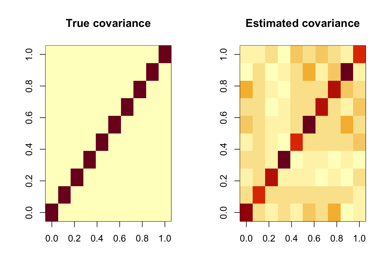
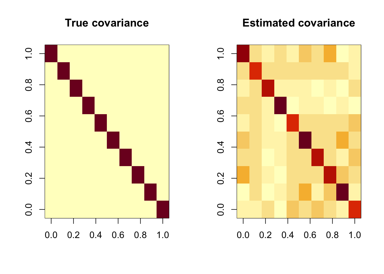
Obtain the estimated covariance matrix \(\hat{\Sigma}\) and check it is close to the true parameter \(\Sigma\). Comparing two p x p matrix is a bit tricky as the matrix is too huge to compare by eyes. Can we use visualisation?
Click for solution
Sigmahat <- cov(dat)
par(mfrow=c(1, 2))
image(t(Sigma), main = "True covariance")
image(t(Sigmahat), main = "Estimated covariance")
However, those images are not what we expected. Why? because image() in R turns the matrix upside down. So we need to make it reverse.
par(mfrow=c(1, 2))
image(Sigma[,nrow(Sigma):1], main = "True covariance")
image(Sigmahat[,nrow(Sigmahat):1], main = "Estimated covariance")
Exercise 2 (Distance measure)
Going back to the high school math, let’s consider two dots in a coordinate plane.
Task 2a
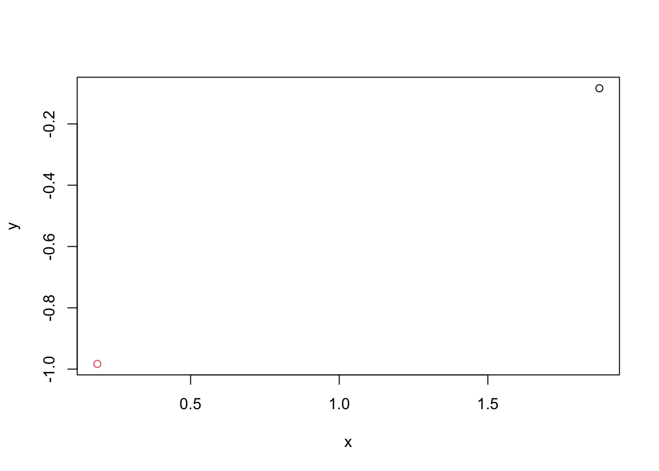
Generate the bivariate Gaussian data \(\boldsymbol{X} \sim N(\boldsymbol{0}, \boldsymbol{I}_p)\) with \(n=2\) and \(p=2\), and point two observations in a coordinate plan (plotting dots) using different colours, where the first variable corresponds to \(x\) axis and the second variable corresponds to \(y\) axis. (If you have no idea how to add a dot in a plot, run ?points in console to get a hint.)
Click for solution
n <- 2
p <- 2
mu <- rep(0, p)
Sigma <- diag(p)

set.seed(2023)
dat <- mvrnorm(n = n, mu = mu, Sigma = Sigma)
obs1 <- dat[1,]
obs2 <- dat[2,]

plot(obs1[1], obs1[2], type="p", xlab="x", ylab="y", xlim=range(dat[,1]), ylim=range(dat[,2]))
points(obs2[1], obs2[2], col=2)
Task 2b
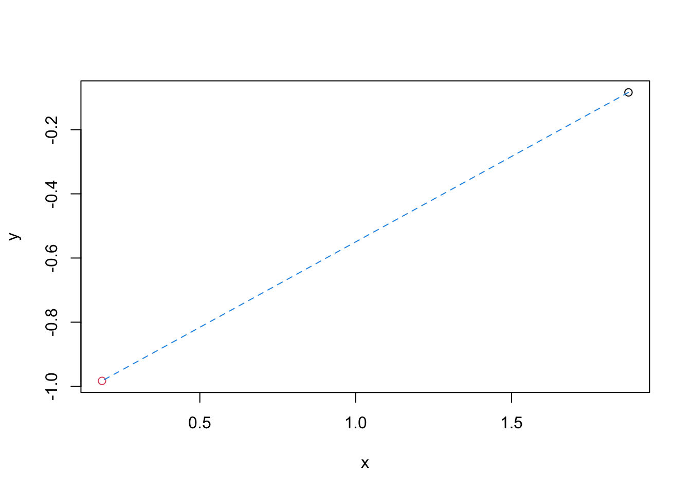
Plot the shortest path between these two dots and find the Euclidean distance. (running ?segments would be helpful.)
Click for solution
plot(obs1[1], obs1[2], type="p", xlab="x", ylab="y", xlim=range(dat[,1]), ylim=range(dat[,2]))
points(obs2[1], obs2[2], col=2)
segments(x0=obs1[1], y0=obs1[2], x1=obs2[1], y1=obs2[2], col=4, lty=2)
# 1) calculating by hand using the formula
d <- sqrt((obs2[1]-obs1[1])^2 + (obs2[2]-obs1[2])^2)
d
## [1] 1.91336# 2) using the "norm" function in R
norm(obs1-obs2, type="2")## [1] 1.91336
Task 2c
Now, we will look at how the Euclidean distance is defined in multi-dimensional setting e.g. p is greater than 2. Generate the multivariate Gaussian data \(\boldsymbol{X} \sim N(\boldsymbol{0}, \boldsymbol{I}_p)\) with \(n=2\) and \(p=10\), and find the Euclidean distance between two observations. For the definition of the Euclidean distance, please check HERE.
Click for solution
n <- 2
p <- 10
mu <- rep(0, p)
Sigma <- diag(p)

set.seed(2023)
dat <- mvrnorm(n = n, mu = mu, Sigma = Sigma)
obs1 <- dat[1,]
obs2 <- dat[2,]

# 1) calculating by hand using the formula
d <- sqrt(sum((obs2-obs1)^2))
d
## [1] 3.561489# 2) using the "norm" function in R
norm(obs1-obs2, type="2")## [1] 3.561489
Exercise 3 (Eigendecomposition)
For every \(p \times p\) symmetric matrix can be decomposed as \[\begin{equation*} A = P \Lambda P^\top \end{equation*}\] where the columns of \(P\) are orthonormal eigenvectors of \(A\) and \(\Lambda\) is a diagonal matrix whose entries are the eigenvalues of \(A\).
We are going to use a (symmetric) covariance matrix for \(A\). Let’s generate a covariance matrix of \(X\) where \(\boldsymbol{X} \sim N(\boldsymbol{0}, \boldsymbol{I}_p)\) with \(n=100\) and \(p=3\).
n <- 100
p <- 3
mu <- rep(0, p)

set.seed(2023)
X <- mvrnorm(n = n, mu = mu, Sigma = diag(p))
Sigmahat <- cov(X)
Task 3a
Perform the eigendecomposition of the estimated covariance matrix using eigen() function in R. Run ?eigen to see how to use the function. Find the matrices \(P\) and \(\Lambda\) from the results.
Click for solution
eigdec <- eigen(Sigmahat)
eigdec
## eigen() decomposition
## $values
## [1] 0.9993261 0.9762688 0.8677176
##
## $vectors
##            [,1]       [,2]       [,3]
## [1,] -0.6734003 0.69786123  0.2439707
## [2,] -0.2508940 0.09469287 -0.9633719
## [3,] 0.6954022 0.70994575 -0.1113230Lambda <- diag(eigdec$values)
Lambda## [,1] [,2] [,3]
## [1,] 0.9993261 0.0000000 0.0000000
## [2,] 0.0000000 0.9762688 0.0000000
## [3,] 0.0000000 0.0000000 0.8677176P <- eigdec$vectors
P## [,1] [,2] [,3]
## [1,] -0.6734003 0.69786123 0.2439707
## [2,] -0.2508940 0.09469287 -0.9633719
## [3,] 0.6954022 0.70994575 -0.1113230
Task 3b
Recall \(A\) is equal to the covariance matrix of \(X\) we used. Then now check if \(A = P \Lambda P^\top\) is right, by comparing \(A\) and \(P \Lambda P^\top\).
Click for solution
Sigmahat## [,1] [,2] [,3]
## [1,] 0.980263399 0.02940887 -0.007849181
## [2,] 0.029408874 0.87697539 -0.015664487
## [3,] -0.007849181 -0.01566449 0.986073701P%*%Lambda%*%t(P)## [,1] [,2] [,3]
## [1,] 0.980263399 0.02940887 -0.007849181
## [2,] 0.029408874 0.87697539 -0.015664487
## [3,] -0.007849181 -0.01566449 0.986073701sum(Sigmahat-P%*%Lambda%*%t(P))## [1] -0.0000000000000003833739Task 3c
Find the eigenvalues of the inverse matrix of the covariance matrix of \(X\). Compare it with the eigenvalues of the covariance matrix of \(X\). Can you find any clear relationship between two vectors?
Click for solution
e1 = eigen(Sigmahat)$values

e2 = eigen(solve(Sigmahat))$values

e2
## [1] 1.152449 1.024308 1.000674sort(1/e1, decreasing = T)## [1] 1.152449 1.024308 1.000674
Exercise 4 (Singular Value Decomposition)
Unlike eigendecomposition requires the matrix should be a square matrix (dimension is e.g. \(p \times p\)), singular value decomposition can be applied to non-square matrix e.g. \(n \times p\).
Any \(n \times p\) matrix can be decomposed into three matrices;
\[\begin{equation} X_{n \times p} = U_{n \times p} D_{p \times p} V^\top_{p \times p}, \end{equation}\] where \(D\) is a diagonal matrix with \(d_1 \geq \cdots \geq d_p \geq 0\) and \(U\), \(V\) both have orthonormal columns with \(U^\top U=V^\top V=\mathbf{I}\).
Note that columns of \(X\) are centred and \[\begin{align*} &X V = U D V^\top V = U D \\ &Xv_j = d_ju_j, \quad j=1, \ldots, p \end{align*}\]
Task 4a
Perform the singular value decomposition of the \(X_{n \times p}\) matrix using svd() function in R. Be careful, we will centre the matrix \(X\) by the R command scale. Run ?svd to see how to use the function. Find the matrices \(U\), \(D\) and \(V\) from the results. And check \(X = UDV^\top\) by comparing \(X\) and \(UDV^\top\).
Click for solution
X1 <- scale(X)
svdec <- svd(X1)

U <- svdec$u
V <- svdec$v
D <- diag(svdec$d)

range(X1-U%*%D%*%t(V))
## [1] -0.00000000000001565414 0.00000000000001543210
Task 4b
Check if the matrices \(U\) and \(V\) both have orthonormal columns i.e. \(U^\top U = V^\top V = \mathbf{I}\) from the results.
Click for solution
round(t(U)%*%U, 10)## [,1] [,2] [,3]
## [1,] 1 0 0
## [2,] 0 1 0
## [3,] 0 0 1round(t(V)%*%V, 10)## [,1] [,2] [,3]
## [1,] 1 0 0
## [2,] 0 1 0
## [3,] 0 0 1
Task 4c
Let’s compare the singular value matrix \(D\) with the eigenvalues obtained in Exercise 3. Compare \(D/\sqrt{n-1}\) and \(\sqrt{\Lambda}\), where the square root transformation for \(\Lambda\) and the division for \(D\) are applied to all elements of the corresponding matrix. Why the results are the same?
Click for solution
eigdec <- eigen(cov(X1))
Lambda <- diag(eigdec$values)

sqrt(Lambda)
## [,1] [,2] [,3]
## [1,] 1.019613 0.0000000 0.000000
## [2,] 0.000000 0.9967415 0.000000
## [3,] 0.000000 0.0000000 0.983309D/sqrt(n-1)## [,1] [,2] [,3]
## [1,] 1.019613 0.0000000 0.000000
## [2,] 0.000000 0.9967415 0.000000
## [3,] 0.000000 0.0000000 0.983309