Workshop: Hierarchical clustering
This exercise involves the illustration of hierarchical clustering and model based clustering using Iris data. We will understand the algorithm of hierarchical clustering and how it can be visualised in a different way. We will also learn how to use agglomerative coefficient to select appropriate linkage in Hierarchical clustering. At the end of the workshop, we will understand why the model based clustering can be a stable alternative to non-model based clustering. You will learn how to implement the models in R.
Hierarchical clustering
iris.scaled <- scale(iris[, -5])The next step is to compute the Euclidean distances and hierarchical clustering with complete linkage (other linkage such as single, average, centroid, ward.D can also be used).
# Compute distances and hierarchical clustering
dd <- dist(iris.scaled, method = "euclidean")
hc <- hclust(dd, method = "complete")
hc
##
## Call:
## hclust(d = dd, method = "complete")
##
## Cluster method : complete
## Distance : euclidean
## Number of objects: 150We can visualise the object by using a dendrogram. This will enable us to determine the point to cut the tree, resulting in the number of clusters.
dendros <- as.dendrogram(hc)
plot(dendros, main = "Iris data - Complete linkage",
     ylab = "Height")
abline(h=0.2, lty = 2, col="red")
abline(h=0.428, lty = 2, col="blue")#point 116 and 142 are merged
Hs <- hc$height[(length(hc$height)-4):length(hc$height)]
abline(h=Hs, col=3, lty=2)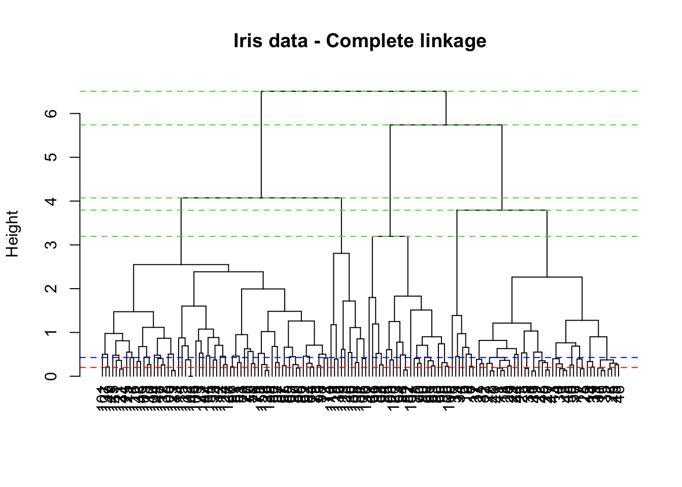
The height axis on the dendrogram displays the dissimilarity between observations and/or clusters. The horizontal bars indicate the point at which two clusters/observations are merged. Thus, observations 137 and 149 are merged at a distance (height) of 0.2 (see the red line and carefully read the numbers on the x-axis). Also, observations 111 and 116 are merged at a height of about 0.428 (see the blue line).
Dissimilarity scores between merged clusters only increases as we run the algorithm. In other words, we can draw a proper dendrogram, where the height of a parent is always higher than height of its daughters. This property is called no inversion property which is illustrated with dashed green lines in the plot.
Visualisation of the plot above can be improved by using the fviz_cluster() and fviz_dend() function in factoextra package (we will be able to see the observations number clearly) as follows:
library(factoextra)

fviz_cluster(list(data=iris.scaled, cluster=cutree(hc, 3)), ellipse.type = "norm")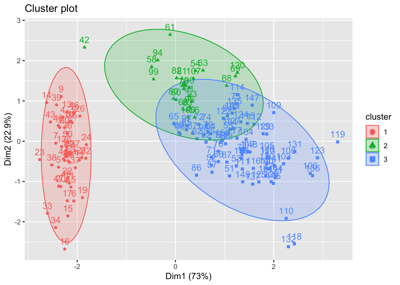
fviz_dend(hc, k = 3, # Cut in three groups
          cex = 0.5, # label size
          k_colors = c("#2E9FDF", "#00AFBB", "#E7B800"),
          color_labels_by_k = TRUE, # color labels by groups
          ggtheme = theme_gray() # Change theme
)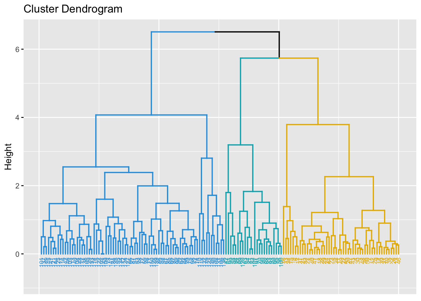
We can also examine the number of observations in each of the three clusters.
hcut <- cutree(hc, k = 3)
table(hcut)
## hcut
## 1 2 3
## 49 24 77The aggregate() function can be used to compute the mean of each variables by clusters using original data.
aggregate(iris[, -5], by=list(cluster=hcut), mean)## cluster Sepal.Length Sepal.Width Petal.Length Petal.Width
## 1 1 5.016327 3.451020 1.465306 0.244898
## 2 2 5.512500 2.466667 3.866667 1.170833
## 3 3 6.472727 2.990909 5.183117 1.815584We have used complete linkage. For practical purposes, we may want to examine which of the three linkages (we learn about three linkages in the lecture but they are more than three) is best for our data set. We can use the agnes function (acronym for Agglomerative Nesting) from cluster package to do this. This will compute the so called agglomerative coefficient (ac). The AC measures the dissimilarity of an object to the first cluster it joins, divided by the dissimilarity of the final merger in the cluster analysis, averaged across all samples. The AC represents the strength of the clustering structure; values closer to 1 indicates that clustering structure is more balanced while values closer to 0 suggests less well balanced clusters. The higher the value, the better.
library(cluster)
m <- c("average","single","complete")
names(m) <- c("average","single","complete")
# function to compute coefficient
ac <- function(x){
  agnes(iris.scaled, method = x)$ac
}
We can now use the map function from tidyverse package, specifically map_dbl() to obtain the agglomerative coefficients. Note that the map functions transform their input by applying a function to each element of a list or atomic vector (use Google to check the meaning of atomic vector) and returning an object of the same length as the input.
library(tidyverse)
 map_dbl(m,ac)
## average single complete
## 0.9035705 0.8023794 0.9438858The highest ac value is 94.4%. So, complete linkage is the best choice among the three. We are on course with the use of complete linkage.
We can also visualise the data using phylogenic-like tree as we did in the lecture note. You will need to load the package igraph and combine it with fviz_dend() function to do this.
Further visualisation using phylogenic-like tree can be accomplished as follows:
library(igraph)
fviz_dend(hc, k = 3, k_colors = "jco", type = "phylogenic", repel = TRUE)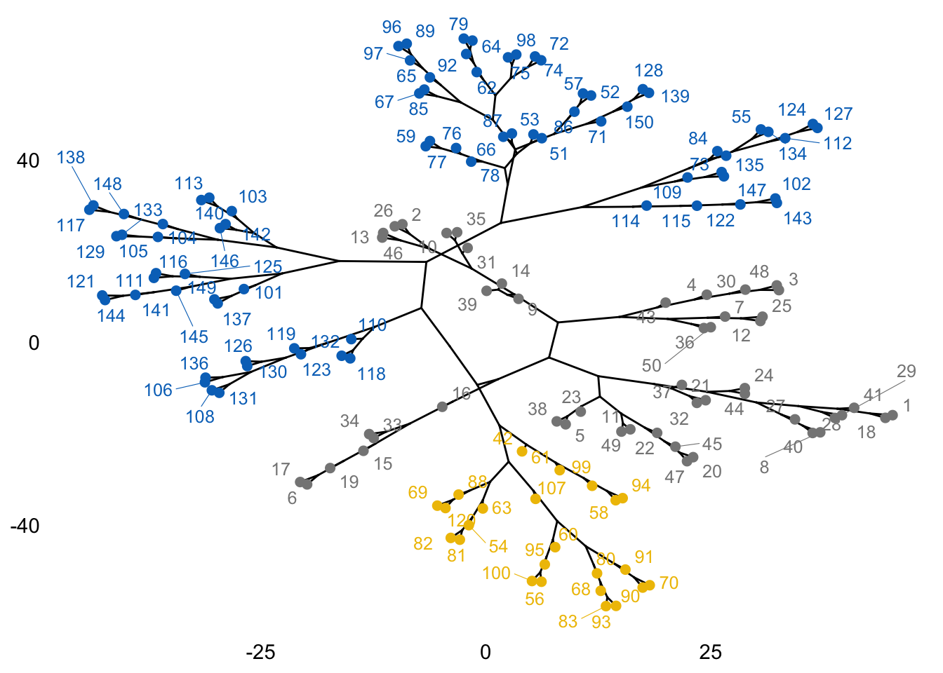
We can compare original species labels with our results from Hierarchical clustering
dd <- cbind(iris, cluster=hcut)
table(dd$Species,dd$cluster)
##
## 1 2 3
## setosa 49 1 0
## versicolor 0 21 29
## virginica 0 2 48Overall, 78.7% correct classification is obtained from the algorithm (that is, ((49+21+48)/150)*100 = 78.7%)
Model-based clustering
The clustering methods that we have discussed so far neither involve any sort of model nor is based on a density estimate. Model-based clustering considers the data as coming from a distribution that is mixture of two or more clusters. Each cluster \(k\) is modelled by the normal or Gaussian distribution which is characterised by the parameters:
- \(\mu_{k}:\) mean vector
- \(\Sigma_{k}:\) covariance matrix
- \(p_{k}\) associated probability in the mixture. Each point has a probability of belonging to each cluster.
The model parameters can be estimated using the Expectation-Maximisation (EM) algorithm initialised by hierarchical model-based clustering. Each cluster \(k\) is centred at the means \(\mu_{k}\), with increased density for points near the mean. The method has been implemented in the mclust package in R.
Since the model is based on maximum likelihood estimation, criterion such as BIC (Bayesian Information Criterion) and AIC (Akaike Information Criterion) can be used for the selection of the number of clusters.
\[AIC = -2logL +2p\] \[BIC = -2logL +log(n)p\] where \(logL\) is the model log-likelihood, \(p\) is the number of parameters and \(n\) is the number of observations. In general, we want these criteria to be small. A model with the smallest value of the criterion is selected as the best.
BIC is often used for selecting the number of clusters. If you did not use this criterion for variable selection in your Machine Learning module, please see here.
The implementation of BIC supports the higher the value the better. This is because the BIC implemented in mclust is defined with a positive sign. A model is fitted for varying number of clusters and the number \(k\) that gives the highest BIC value is selected for the data.
Let us use the package on iris data set.
library(mclust)
iris.scaled <- scale(iris[, -5]) # Standardise the data
mc <- Mclust(iris.scaled, G = 3) # Model-based-clustering, G=3 indicates a request for 3 clusters
summary(mc)
## ----------------------------------------------------
## Gaussian finite mixture model fitted by EM algorithm
## ----------------------------------------------------
##
## Mclust VVV (ellipsoidal, varying volume, shape, and orientation) model with 3
## components:
##
## log-likelihood n df BIC ICL
## -288.5255 150 44 -797.519 -800.7391
##
## Clustering table:
## 1 2 3
## 50 45 55The result indicates that there are 50 observations in cluster 1, 45 in cluster 2 and 55 in cluster 3.
We can examine the variables created within object mc:
names(mc)## [1] "call" "data" "modelName" "n"
## [5] "d" "G" "BIC" "loglik"
## [9] "df" "bic" "icl" "hypvol"
## [13] "parameters" "z" "classification" "uncertainty"The value that is of utmost importance in the object created is classification. These are the newly created clusters.
mc$classification## [1] 1 1 1 1 1 1 1 1 1 1 1 1 1 1 1 1 1 1 1 1 1 1 1 1 1 1 1 1 1 1 1 1 1 1 1 1 1
## [38] 1 1 1 1 1 1 1 1 1 1 1 1 1 2 2 2 2 2 2 2 2 2 2 2 2 2 2 2 2 2 2 3 2 3 2 3 2
## [75] 2 2 2 3 2 2 2 2 2 3 2 2 2 2 2 2 2 2 2 2 2 2 2 2 2 2 3 3 3 3 3 3 3 3 3 3 3
## [112] 3 3 3 3 3 3 3 3 3 3 3 3 3 3 3 3 3 3 3 3 3 3 3 3 3 3 3 3 3 3 3 3 3 3 3 3 3
## [149] 3 3
As a small task, use the table() function in R to compare the true class labels to the class labels obtained from mclust. Does this result offer any improvement over the K-means clustering results in Workshop 3?
##
##               1  2  3
##   setosa     50  0  0
##   versicolor  0 45  5
##   virginica   0  0 50
If you implemented this correctly, then Setosa is correctly classified (50 out of 50 correctly classified). 5 observations are misclassified in Versicolor (45 out of 50 correctly classified). Overall, 97% correct classification is obtained under the model-based clustering, whereas it was 88% under K-medoids and 83.3% under K-means.
You can obtain four different types of plot from the mc object that was created.
Model-based clustering plots:
1: BIC
2: classification
3: uncertainty
4: density
We can plot the classification as follows:
plot(mc, what = "classification")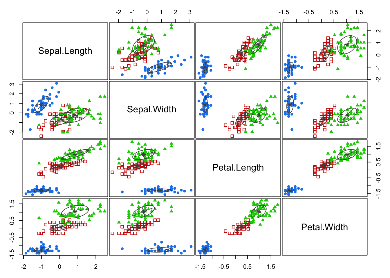
We can identify the 5 observations that were misclassified and calculate the classification error rate as follows.
classError(mc$classification, iris[,5])## $misclassified
## [1] 69 71 73 78 84
##
## $errorRate
## [1] 0.03333333
Observe that the mclust output contains the following comment: "Mclust VVV (ellipsoidal, varying volume, shape, and orientation) model with 3 components:". This is based on the parametrisation of the covariance matrix, \(\Sigma_{k}\) used. The available model options in mclust package, are represented by identifiers including:
EII, VII, EEI, VEI, EVI, VVI, EEE, EEV, VEV and VVV. So, VVV (geometric features: shape, volume, orientation) has been used for our example. The first identifier refers to volume, the second to shape and the third to orientation. E stands for “equal”, V for “variable” and I for “coordinate axes”. VEI, for example, implies that the clusters have variable volume, the same shape and orientation equal to coordinate axes. EEE means that the clusters have the same volume, shape and orientation in p-dimensional space. To find out more about model options, type ?mclustModelNames in R studio console.
To enforce VVV as a model option, for example, you can do the following:
mc_option <- Mclust(iris.scaled, G = 3, modelNames = "VVV")Now, let us try to compare the performance of model options VVI, EVE and VEI to VVV.
You are required to fit the models using the three model options, create a classification table and compare the percentage of correct classification with what we obtained for VVV.
mc_option_VVI <- Mclust(iris.scaled, G = 3, modelNames = "VVI")
table(iris[,5], mc_option_VVI$classification)
##
## 1 2 3
## setosa 50 0 0
## versicolor 0 49 1
## virginica 0 14 36(50+49+36)/150## [1] 0.9mc_option_EVE <- Mclust(iris.scaled, G = 3, modelNames = "EVE")
table(iris[,5], mc_option_EVE$classification)##
## 1 2 3
## setosa 50 0 0
## versicolor 0 50 0
## virginica 0 16 34(50+50+34)/150## [1] 0.8933333mc_option_VEI <- Mclust(iris.scaled, G = 3, modelNames = "VEI")
table(iris[,5], mc_option_VEI$classification)##
## 1 2 3
## setosa 50 0 0
## versicolor 0 48 2
## virginica 0 4 46(50+48+46)/150## [1] 0.96mc_option_VVV <- Mclust(iris.scaled, G = 3, modelNames = "VVV")
table(iris[,5], mc_option_VVV$classification)##
## 1 2 3
## setosa 50 0 0
## versicolor 0 45 5
## virginica 0 0 50(50+45+50)/150## [1] 0.9666667Clearly, the automatically selected model option, VVV is the best with 97% classification accuracy. This is followed by VEI at 96% accuracy. The worst is VVI at 90%, although it is still better than all the previous clustering methods (K-means, K-medoids and Hierarchical).
As stated previously, one can use the BIC criterion (higher values are desirable) to select the number of clusters (G). Consider the case below:
mc_bic <- Mclust(iris.scaled, G = 3)
mc_bic$BIC
## Bayesian Information Criterion (BIC):
## EII VII EEI VEI EVI VVI EEE
## 3 -1214.525 -1222.844 -1029.733 -995.8343 -1014.515 -961.3205 -849.6448
## VEE EVE VVE EEV VEV EVV VVV
## 3 -822.076 -862.9077 -828.8731 -875.3724 -797.5483 -872.7515 -797.519
##
## Top 3 models based on the BIC criterion:
## VVV,3 VEV,3 VEE,3
## -797.5190 -797.5483 -822.0760You will observe that the results included the top 3 model options based on the BIC criterion.
Now, let’s use the BIC criterion to select the number of clusters from the set G = {2, 3, 4, 5}.
mc_bic2 <- Mclust(iris.scaled, G = 2)
mc_bic2$BIC
## Bayesian Information Criterion (BIC):
## EII VII EEI VEI EVI VVI EEE VEE
## 2 -1344.053 -1325.273 -1259.646 -1172.96 -1223.986 -1074.229 -904.775 -873.0048
## EVE VVE EEV VEV EVV VVV
## 2 -906.9282 -880.7933 -873.659 -802.5253 -875.0084 -790.6956
##
## Top 3 models based on the BIC criterion:
## VVV,2 VEV,2 VEE,2
## -790.6956 -802.5253 -873.0048mc_bic3 <- Mclust(iris.scaled, G = 3)
mc_bic3$BIC## Bayesian Information Criterion (BIC):
## EII VII EEI VEI EVI VVI EEE
## 3 -1214.525 -1222.844 -1029.733 -995.8343 -1014.515 -961.3205 -849.6448
## VEE EVE VVE EEV VEV EVV VVV
## 3 -822.076 -862.9077 -828.8731 -875.3724 -797.5483 -872.7515 -797.519
##
## Top 3 models based on the BIC criterion:
## VVV,3 VEV,3 VEE,3
## -797.5190 -797.5483 -822.0760mc_bic4 <- Mclust(iris.scaled, G = 4)
mc_bic4$BIC## Bayesian Information Criterion (BIC):
## EII VII EEI VEI EVI VVI EEE
## 4 -1177.163 -1139.392 -1044.112 -965.1348 -1054.223 -967.7021 -862.7323
## VEE EVE VVE EEV VEV EVV VVV
## 4 -821.5149 -902.9964 -881.127 -930.1693 -821.4057 -941.9898 -847.2777
##
## Top 3 models based on the BIC criterion:
## VEV,4 VEE,4 VVV,4
## -821.4057 -821.5149 -847.2777mc_bic5 <- Mclust(iris.scaled, G = 5)
mc_bic5$BIC## Bayesian Information Criterion (BIC):
## EII VII EEI VEI EVI VVI EEE VEE
## 5 -1135.642 -1107.791 -958.6219 -905.0241 -983.5054 -928.1301 -821.5159 NA
## EVE VVE EEV VEV EVV VVV
## 5 -901.9539 -853.4148 -877.2201 -837.6111 NA -893.2973
##
## Top 3 models based on the BIC criterion:
## EEE,5 VEV,5 VVE,5
## -821.5159 -837.6111 -853.4148The results show that \(G = 2\) has the highest BIC value with the model option VVV. The next is \(G = 3\). Although the best number of clusters is chosen to be two, this is not far from the three clusters that we have used for the data set (the natural subgroups for the data are indeed three).